I think the method of maximum entropy to obtain probability distributions is so cool. You take a few knowns or constraints, and then maximize information entropy subject to these conditions and voila! you have a unique probability distribution. The cool thing is that these maximum entropy distributions are quite common, so this is a neat way of re-deriving many of the distibutions we encounter day-to-day. For me that alone is worth the cost of entry. But from an information-theoretic perspective, these will be the least biased prior distributions (we maximize our ignorance) so subsequent experiments a la Bayes’ theorem will maximize the information gained. Moreover, many physical patterns found in nature tend toward maximum entropy probability distributions. So even as a way to understand the world, maximum entropy is a very useful and deep tool.
Here are some common probability distributions and how to derive them from the principle of maximum entropy.
Table of Contents
- Discrete uniform distribution
- Continuous uniform distribution
- Cauchy distribution
- Exponential distribution
- Gaussian distribution
- Bernoulli distribution
- Binomial distribution
For the discrete case, consider \(N\) different possibilities, e.g.
\(i \in X = \{1,2,\ldots,N\}\), and we have no other information other
than the constraint that the probabilities \(p_i\) sum to 1. In this case,
we maximize
\[H(p) = -\sum_{i=1}^N p_i \ln p_i\]
subject to
\[\sum_{i=1}^N p_i = 1\]
by the method of Lagrange multipliers. So we
take the derivative with respect to \(p_i\) of the Lagrangian
\[\begin{aligned}
\frac{\partial J(p,\lambda_0)}{\partial p_i} &= \frac{\partial}{\partial p_i} \left(-\sum_{i=1}^N p_i \ln p_i + \lambda_0 \left(\sum_{i=1}^N p_i - 1\right)\right) \\
&= -\ln p_i - 1 + \lambda_0 = 0\end{aligned}\]
and we set the result
equal to zero, as this is a maximization. Note that the second
derivative is negative, indicating we are at a maximum, e.g.
\[\frac{\partial^2 J(p,\lambda_0)}{\partial p_i^2} = - 1/ p_i\]
and \(p_i\) is always positive. Therefore, we find that
\[p_i = \exp \left(\lambda_0 - 1\right)\]
and plugging into our normalization expression yields
\[\begin{aligned}
\sum_{i=1}^N p_i &= 1 \\
\sum_{i=1}^N \exp \left(\lambda_0 - 1\right) &= 1 \\
N \exp \left(\lambda_0 - 1\right) &= 1 \\
\exp \left(\lambda_0 - 1\right) &= 1/N\end{aligned}\]
which yields the discrete uniform probability distribution,
\[p_i = 1/N\]
This is the maximum entropy distribution for the case with \(N\) possible
outcomes with no other information given (other than our probabilities
are normalized).
This is similar, to the discrete case we just saw, but now assume that
the random variable \(x\) can take any value in \([a,b]\). Then we want to
maximize
\[H(p(x)) = - \int_a^b p(x)\ln p(x) dx\]
subject to
\[\int_a^b p(x) dx = 1\]
which gives us our Lagrangian
\[J(p(x),\lambda_0) = - \int_a^b p(x)\ln p(x) dx + \lambda_0 \left(\int_a^b p(x) dx - 1\right)\]
differentiating the above with respect to \(p(x)\) and setting to zero
gives
\[\begin{aligned}
\frac{\partial J(p(x),\lambda_0)}{\partial p(x)} &= \frac{\partial}{\partial p(x)} \left(- \int_a^b p(x)\ln p(x) dx + \lambda_0 \left(\int_a^b p(x) dx - 1\right)\right) \\
&= -\ln p(x) - 1 + \lambda_0 = 0.
\end{aligned}\]
which gives us an expression for \(p(x)\) as
\[p(x) = \exp \left(\lambda_0 - 1\right)\]
Like before, we can solve for \(\lambda_0\) by plugging the result back in our
normalization expression to get
\[\begin{aligned}
\int_a^b p(x) dx &= 1 \\
\int_a^b \exp \left(\lambda_0 - 1\right) dx &= 1 \\
\exp \left(\lambda_0 - 1\right) \int_a^b dx &= 1 \\
\exp \left(\lambda_0 - 1\right) (b - a) &= 1 \\
\exp \left(\lambda_0 - 1\right) &= \frac{1}{(b-a)}\end{aligned}\]
yielding
\[p(x) = \frac{1}{(b-a)}\]
which is the continuous
uniform distribution over \([a,b]\).
Cauchy distribution
The Cauchy distribution can be obtained in a similar way to the
continuous uniform distribution, but in a particular geometric
configuration. Consider the relationship between and angle \(\theta_k\)
and a point \(x_k\) on a line some distance away, as illustrated in
the diagram below. In this
case we want to consider the case where our random variable \(\theta\) is
an angle is on \([-\pi/2, \pi/2]\) and we don’t know anything else about
the underlying distribution other than it is normalized. So we maximize
\[H(p(\theta)) = - \int_{-\pi/2}^{\pi/2} p(\theta)\ln p(\theta) d\theta\]
subject to
\[\int_{-\pi/2}^{\pi/2} p(\theta) d\theta = 1\]
Now, from the
previous section we know that the MaxEnt procedure would result in
\(p(\theta) = 1/\pi\), which is obviously not the Cauchy distribution. To
get the Cauchy distribution, we actually want to consider this case but
in terms of a distribution over \(x\), where the relationship between \(x\)
and \(\theta\) is given by \(h \tan \theta = x - x_0\), where \(h\) and \(x_0\)
are arbitrary parameters.
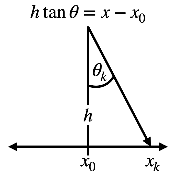
Relationship between \(\theta\) and \(x\). Here we want to consider the
case where we don’t know anything about the underlying probability
distribution of \(\theta\) other than that it is supported on
\([-\pi/2, \pi/2]\) and that is is normalized, and we want this result as
a distribution on \(x\). \(h\) and \(x_0\) are arbitrary
parameters.
Since we have the relationship between \(\theta\) and \(x\), and the
relationship is defined over \(\theta \in [-\pi/2,\pi/2]\), we can do a
change of variables to get \(p(x)\) instead of \(p(\theta)\) and then carry
out the maximization of entropy. To do the change of variables, we need
\[\begin{aligned}
h \tan \theta &= x - x_0 \\
h \sec^2 \theta~d \theta &= dx \\
h (\tan^2 \theta + 1)~d \theta &= dx \\
h \left[\left(\frac{x - x_0}{h}\right)^2 + 1\right]~d \theta &= dx \\
\frac{1}{h}\left[\left(x - x_0\right)^2 + h^2 \right]~d\theta &= dx \\
d\theta &= \frac{h}{\left(\left(x - x_0\right)^2 + h^2 \right)} dx\end{aligned}\]
so that
\[p(\theta) = p(x) \left| \frac{dx}{d\theta}\right| = p(x) \frac{1}{h}\left[\left(x - x_0\right)^2 + h^2 \right]\]
For the limits on integration, we can easily see that
\(\tan (\pi/2) \to \infty\) and \(\tan (-\pi/2) \to -\infty\)
so \(x \in (-\infty,\infty)\). All together, we now want to maximize
\[\begin{aligned}
H(p(\theta)) &= - \int_{-\pi/2}^{\pi/2} p(\theta)\ln p(\theta) d\theta \\
H(p(x)) &= - \int_{-\infty}^{\infty} \frac{p(x) \left(\left(x - x_0\right)^2 + h^2 \right)}{h}\ln \left[ \frac{p(x)\left(\left(x - x_0\right)^2 + h^2 \right)}{h}\right] \frac{h}{\left(\left(x - x_0\right)^2 + h^2 \right)} dx \\
&= - \int_{-\infty}^{\infty} p(x) \ln \left[ \frac{p(x)\left(\left(x - x_0\right)^2 + h^2 \right)}{h}\right]dx \\
&= - \int_{-\infty}^{\infty} p(x) \ln p(x) dx - \int_{-\infty}^{\infty} p(x) \ln \left[\frac{\left(\left(x - x_0\right)^2 + h^2 \right)}{h}\right]dx
\end{aligned}\]
subject to \(\int_{-\infty}^{\infty} p(x) dx = 1\) therefore, our
Lagrangian is
\[\begin{aligned}
J(p(x),\lambda_0) &= - \int_{-\infty}^{\infty} p(x) \ln p(x) dx \\
&\quad - \int_{-\infty}^{\infty} p(x) \ln \left[\frac{\left(\left(x - x_0\right)^2 + h^2 \right)}{h}\right]dx \\
&\quad + \lambda_0 \left(\int_{-\infty}^{\infty} p(x) dx - 1\right)
\end{aligned}\]
and carrying out the maximization yields
\[\frac{\partial J(p(x),\lambda_0)}{\partial p(x)} = -1 - \ln p(x) - \ln \left[\frac{\left(\left(x - x_0\right)^2 + h^2 \right)}{h}\right] + \lambda_0 = 0\]
which gives
\[\begin{aligned}
p(x) &= \exp \left(\lambda_0 - 1 - \ln \left[\frac{\left(\left(x - x_0\right)^2 + h^2 \right)}{h}\right] \right) \\
&= \frac{h}{\left(\left(x - x_0\right)^2 + h^2 \right)} \exp (\lambda_0 - 1)
\end{aligned}\]
substituting this into the normalization condition allows us to
eliminate the \(\lambda_0\)
\[\begin{aligned}
\int_{-\infty}^{\infty} \frac{h}{\left(\left(x - x_0\right)^2 + h^2 \right)} \exp (\lambda_0 - 1)dx &= 1 \\
\exp (\lambda_0 - 1) \int_{-\infty}^{\infty} \frac{h}{\left(\left(x - x_0\right)^2 + h^2 \right)}dx &= 1 \\
\exp (\lambda_0 - 1) \pi &= 1 \\
\exp (\lambda_0 - 1) &= 1/\pi
\end{aligned}\]
therefore, we get
\[p(x) = \frac{h}{\pi\left(\left(x - x_0\right)^2 + h^2 \right)}\]
So for sampling random angles and not knowing anything about the
underlying distribution (e.g. \(\theta\) is continuous uniform), we see
that the resulting distribution over \(x\) is a Cauchy distribution, when
\(x\) and \(\theta\) have the relationship illustrated above.
Exponential distribution
Now extend the continuous distribution to the case where we have a known
expected value of \(x = \mu\). We will limit ourselves to the support
\([0,\infty)\). As before we maximize
\[H(p(x)) = - \int_0^\infty p(x)\ln p(x) dx\]
but now subject to
\[\int_0^\infty p(x) dx = 1, \qquad \int_0^\infty x p(x) dx = \mu\]
which gives us our Lagrangian
\[J(p(x),\lambda_0, \lambda_1) = - \int_0^\infty p(x)\ln p(x) dx + \lambda_0 \left(\int_0^\infty p(x) dx - 1\right) + \lambda_1 \left(\int_0^\infty x p(x) dx - \mu\right)\]
differentiating the above with respect to \(p(x)\) and setting to zero gives
\[\begin{aligned}
\frac{\partial J(p(x),\lambda_0, \lambda_1)}{\partial p(x)} &= \frac{\partial}{\partial p(x)} \left(- \int_0^\infty p(x)\ln p(x) dx + \lambda_0 \left(\int_0^\infty p(x) dx - 1\right)+ \lambda_1 \left(\int_0^\infty x p(x) dx - \mu\right)\right) \\
&= -\ln p(x) - 1 + \lambda_0 +\lambda_1 x = 0.
\end{aligned}\]
which gives us an expression for \(p(x)\) as
\[p(x) = \exp \left(\lambda_0 - 1\right) \exp(\lambda_1 x)\]
this results in the following expressions for our constraints:
\[\int_0^\infty p(x) dx = \exp \left(\lambda_0 - 1\right) \int_0^\infty \exp(\lambda_1 x) dx = \exp \left(\lambda_0 - 1\right) \left(\frac{-1}{\lambda_1}\right) = 1\]
where \(\frac{-1}{\lambda_1} < 0\) in order for the integral to converge.
For the second constraint we have
\[\int_0^\infty x p(x) dx = \exp \left(\lambda_0 - 1\right) \int_0^\infty x \exp(\lambda_1 x) dx = \exp \left(\lambda_0 - 1\right) \left(\frac{1}{\lambda_1^2}\right) = \mu\]
Dividing the two constraints by each other allows us to solve for
\(\lambda_1\):
\[\frac{\exp \left(\lambda_0 - 1\right)}{\exp \left(\lambda_0 - 1\right)}\frac{-1/\lambda_1}{1/\lambda_1^2} = -\lambda_1 = 1/\mu\]
and then from the normalization we get
\[\exp \left(\lambda_0 - 1\right) \int_0^\infty \exp(-x/\mu) dx = \exp \left(\lambda_0 - 1\right) \mu = 1\]
which means \(\exp \left(\lambda_0 - 1\right) = 1/\mu\) and so from
knowing a fixed mean, we obtain the exponential distribution over
\([0,\infty)\)
\[p(x) = \frac{1}{\mu} \exp \left(-\frac{x}{\mu}\right)\]
Gaussian distribution
Now consider the case where we have a known mean \(\mu\) and variance
\(\sigma^2\). We will consider \(x \in (-\infty,\infty)\). Because variance
is the expectation of the squared deviation of a random variable \(x\)
from its mean, it suffices to introduce the constraint
\[\int_{-\infty}^\infty (x - \mu)^2 p(x) dx = \sigma^2\]
which we will consider along with normalization when maximizing the entropy. This leads to the Lagrangian
\[J(p(x),\lambda_0, \lambda_1) = - \int_{-\infty}^\infty p(x)\ln p(x) dx + \lambda_0 \left(\int_{-\infty}^\infty p(x) dx - 1\right) + \lambda_1 \left(\int_{-\infty}^\infty (x- \mu)^2 p(x) dx - \sigma^2\right)\]
which, when differentiated with respect to \(p(x)\) and set equal to zero, yields
\[\frac{\partial J(p(x),\lambda_0, \lambda_1)}{\partial p(x)} = -\ln p(x) - 1 + \lambda_0 +\lambda_1 (x - \mu)^2 = 0\]
which gives us an expression for \(p(x)\) as
\[p(x) = \exp \left(\lambda_0 - 1\right) \exp(\lambda_1 (x-\mu)^2)\]
For the first constraint, we find that
\[\begin{aligned}
\int_{-\infty}^\infty p(x) dx &= 1 \\
\int_{-\infty}^\infty \exp \left(\lambda_0 - 1\right) \exp(\lambda_1 (x-\mu)^2) dx &= 1 \\
\exp \left(\lambda_0 - 1\right) \int_{-\infty}^\infty \exp(\lambda_1 (x-\mu)^2) dx &= 1 \\
\exp \left(\lambda_0 - 1\right) \sqrt{\frac{\pi}{-\lambda_1}} &= 1 \\
\exp \left(\lambda_0 - 1\right) &= \sqrt{\frac{-\lambda_1}{\pi}} .
\end{aligned}\]
And for the second constraint we find
\[\begin{aligned}
\int_{-\infty}^\infty (x - \mu)^2 p(x) dx &= \sigma^2 \\
\int_{-\infty}^\infty \sqrt{\frac{-\lambda_1}{\pi}} (x - \mu)^2 \exp(\lambda_1 (x-\mu)^2) dx &= \sigma^2 \\
\sqrt{\frac{-\lambda_1}{\pi}} \int_{-\infty}^\infty (x - \mu)^2 \exp(\lambda_1 (x-\mu)^2) dx &= \sigma^2 \\
\sqrt{\frac{-\lambda_1}{\pi}} \cdot \frac{1}{2}\sqrt{\frac{\pi}{-\lambda_1^3}} &= \sigma^2 \\
\lambda_1 &= -\frac{1}{2\sigma^2}.
\end{aligned}\]
Which allows us to say that
\[\exp \left(\lambda_0 - 1\right) = \frac{1}{\sqrt{2\pi\sigma^2}}\]
Putting this all together yields the Gaussian, or normal distribution
\[p(x) = \frac{1}{\sqrt{2\pi\sigma^2}}\exp\left(-\frac{(x-\mu)^2}{2\sigma^2}\right)\]
Bernoulli distribution
Moving back to the discrete case, let’s consider when a random variable
\(k\) is either \(0\) or \(1\), i.e. \(k \in \{0,1\}\) and the expected value of
\(k\) is \(\bar{p}\). This results in the Lagrangian
\[J(p_k, \lambda_0, \lambda_1) = -\sum_k p_k \ln p_k + \lambda_0\left(\sum_k p_k - 1\right) + \lambda_1 \left(\sum_k k p_k - \bar{p}\right)\]
Maximizing this Lagrangian gives
\[\frac{\partial J(p_k,\lambda_0)}{\partial p_k} = -1 - \ln p_k + \lambda_0 + \lambda_1 k = 0\]
which yields the probability mass function \(p_k\)
\[p_k = \exp \left(\lambda_0 - 1\right) \exp \left(\lambda_1 k \right)\]
Taking care of the first constraint,
\[\begin{aligned}
\sum_k \exp \left(\lambda_0 - 1\right) \exp \left(\lambda_1 k \right) &= 1 \\
\exp \left(\lambda_0 - 1\right) \sum_k \exp \left(\lambda_1 k \right) &= 1 \\
\exp \left(\lambda_0 - 1\right) &= \frac{1}{\sum_k \exp \left(\lambda_1 k \right)} \\
\exp \left(\lambda_0 - 1\right) &= \frac{1}{\exp \left(\lambda_1 \cdot 0 \right) + \exp \left(\lambda_1 \cdot 1 \right)} \\
\exp \left(\lambda_0 - 1\right) &= \frac{1}{1 + \exp \left(\lambda_1 \right)}
\end{aligned}\]
since \(k\) is either \(0\) or \(1\). Taking care of the second constraint,
\[\begin{aligned}
\sum_k k \cdot \exp \left(\lambda_0 - 1\right) \exp \left(\lambda_1 k \right) &= \bar{p} \\
\exp \left(\lambda_0 - 1\right) \sum_k k \cdot \exp \left(\lambda_1 k \right) &= \bar{p} \\
\frac{\exp \left(\lambda_1 \right)}{1 + \exp \left(\lambda_1 \right)} &= \bar{p}
\end{aligned}\]
again, since \(k\) is either \(0\) or \(1\). Then we can solve for \(\lambda_1\),
\[\lambda_1 = \ln \left( \frac{\bar{p}}{1-\bar{p}} \right)\]
which means that
\[\exp \left(\lambda_0 - 1\right) = \frac{1}{1 + \frac{\bar{p}}{1-\bar{p}}} = (1-\bar{p})\]
Putting this all together we have
\[\begin{aligned}
p_k &= (1 - \bar{p}) \exp \left( k \cdot \ln \left(\frac{\bar{p}}{1-\bar{p}}\right)\right) \\
&= (1 - \bar{p}) \left(\frac{\bar{p}}{1-\bar{p}}\right)^k \\
&= \bar{p}^k (1 - \bar{p})^{k-1} \end{aligned}\]
Which is the Bernoulli distribution
\[p_k = \bar{p}^k (1 - \bar{p})^{k-1}\]
for when \(0 \leq \bar{p} \leq 1\) and \(k\) is either \(0\) or \(1\).
Binomial distribution
This is the case where we compute the probability for having \(N\)
successes in \(M\) trials. The constraint here is the expected number of
successes \(\langle N \rangle\). Note that this will depend on the number
of trials, and since we only care abut the number of successes, and not
the order in which they were taken, we need to use the generalized form
of entropy
\[H(p) = -\sum_N^M p_N \ln \frac{p_N}{m(N)}\]
where \(m(N)\) is the Lebesgue measure, which accounts for the fact that we need to
account for the fact that we are indifferent to the number of ways \(N\)
can be accomplished. This is essentially the prior probability we assign
to the different outcomes. For example, in the uniform distribution we
had no reason to favor one proposition \(p_i\) over another, thus the
principle of indifference led us to assign \(m(i) = 1\) for all \(i\), and
the result led to each outcome being equally likely. But this is not
always the case in combinatoric problems, for example, since (without
replacement) there are 4 ways to pick a unique object out of a set of 4
unique objects, but 6 ways to pick out 2 objects out of the same set. So
we would not expect the probabilities for 2 objects to be on the same
scale as picking out 1 object; our prior information leads us to favor 4
choose 2 over 4 choose 1 – there are more ways it could happen. The
measure \(m(N)\) allows us to account for that.
In other words, for this combinatoric problem,
\[m(N) = M!/N!(M-N)!\]
(As a chemist, I think of \(m(N)\) as event degeneracy.) Now, moving on, we are in addition to the normal entropy and
normalization, constrained by the information
\(\sum_N^M N p_N = \langle N \rangle = \mu\) Therefore, our Lagrangian
reads
\[J(p_N,\ldots) = -\sum_N^M p_N \ln \frac{p_N}{m(N)} + \lambda_0 \left(\sum_N^M p_N - 1\right) + \lambda_1 \left(\sum_N^M N p_N - \mu\right)\]
which leads to the maximization
\[\frac{\partial J}{\partial p_N} = 0 = -1 - \ln \frac{p_N}{m(N)} + \lambda_0 + \lambda_1 N\]
so that
\[\begin{aligned}
p_N &= m(N) \cdot \exp \left(\lambda_0 -1\right) \exp\left( \lambda_1 \right)^N \\
&= \frac{M!}{N!(M-N)!} \exp \left(\lambda_0 -1\right) \exp\left( \lambda_1 \right)^N
\end{aligned}\]
and we chose the combinatoric measure because for each possible number
of successes \(N\), there are \(M!/N!(M-N)!\) different ways of achieving
this given \(M\) trials.
Solving for the first constraint:
\[\begin{aligned}
1 &= \sum_N^M p_N = \exp \left(\lambda_0 -1\right) \sum_N^M \frac{M!}{N!(M-N)!} \exp\left( \lambda_1 \right)^N \cdot (1)^{M-N} \\
&= \exp \left(\lambda_0 -1\right) \exp\left( \lambda_1 + 1\right)^M \\
&\implies \exp \left(\lambda_0 -1\right) = \exp\left( \lambda_1 + 1\right)^{-M}
\end{aligned}\]
where we multiplied by \(1\) to the power of \(M-N\), which just equals one,
in the first line in order to make use of the binomial formula and
eliminate the sum. The inversion in the last line is made possible
because the exponential is always greater than zero.
For the next constraint,
\[\begin{aligned}
\mu &= \sum_N^M N \exp\left( \lambda_1 + 1\right)^{-M} \frac{M!}{N!(M-N)!} \exp\left( \lambda_1 \right)^N \\
&= \exp\left( \lambda_1 + 1\right)^{-M} \sum_N^M N \frac{M!}{N!(M-N)!} \exp\left( \lambda_1 \right)^N \\
&= \exp\left( \lambda_1 + 1\right)^{-M} \cdot \exp \left(\lambda_1\right) \cdot M \cdot \left( \exp\left( \lambda_1 \right) + 1 \right)^{M-1} \\
&= M \cdot \frac{\exp(\lambda_1)}{\exp(\lambda_1) + 1}
\end{aligned}\]
In fairness, I used WolframAlpha to finally eliminate
the sum after the second line. If we let \(p \leftarrow \mu/M\), then we
can finally see that
\[\begin{aligned}
\exp(\lambda_1) = \frac{p}{1-p}\end{aligned}\]
which we can obtain because \(p > 0\).
Okay. Putting it all together now:
\[\exp \left(\lambda_0 -1\right) = \left(\frac{p}{1-p} + 1 \right)^{-M} = \left(\frac{1}{1-p}\right)^{-M} = \left( 1-p \right)^M\]
and
\[\exp \left(\lambda_1 \right)^N = \left(\frac{p}{1-p}\right)^{N} = \left(\frac{1-p}{p}\right)^{-N} = \left(\frac{1}{p} - 1 \right)^{-N}\]
which lets us finally show that
\[p_N = \frac{M!}{N!(M-N)!} \cdot \left( 1-p \right)^M \cdot \left(\frac{1}{p} - 1 \right)^{-N}\]
or, simply,
\[p_N = \frac{M!}{N!(M-N)!} \left(p \right)^{N} \left( 1-p \right)^{M-N}\]
which is the binomial distribution.
Others
There are plenty others, like the Poisson, beta, and von Mises distributions which can be derived in a like manner. I may add more here if I get to it. Until then, check out the table from Wikipedia.
Launch the interactive notebook: 
Table of Contents
- Introduction
- Qubits, gates, and all that
- Make that Hamiltonian!
- A first attempt at a quantum circuit
- A “real” quantum circuit
- A “real” measurement of the energy
- Appendix: All together now
Introduction
The variational quantum eigensolver (VQE) is a hybrid classical-quantum algorithm that variationally determines the ground state energy of a Hamiltonian.
It’s quantum in the sense that the expectation value of the energy is computed via a quantum algorithm, but it is classical in the sense that the energy is minimized with a classical optimization algorithm.
From a molecular electronic structure perspective, it is equivalent to computing the Full Configuration Interaction (FCI) for a given basis.
Quantum computing can be a little unintuitive, so it helps to see a working example. Although we won’t actually do any “real” quantum computing, the methods can be understood from a linear algebra perspective. So that’s what we are going to try and do for the VQE.
The problem we want to tackle is to implement the VQE to compute the energy of molecular hydrogen (H\(_2\)) in a minimal basis. We will base this implementation off the really neat paper
O’Malley, Peter JJ, et al. “Scalable quantum simulation of molecular energies.” Physical Review X 6.3 (2016): 031007.
In the O’Malley paper, they implement the VQE on a real quantum computer to compute the potential energy surface of H\(_2\). The schematic we are going to follow can be seen below, and we are going to implement the “software”.
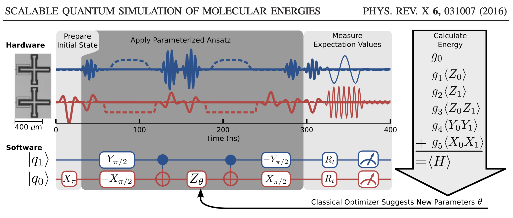
Here’s the big, overarching plan:
- Put the Hamiltonian in the computational (qubit) basis.
- Obtain a variational ansatz to parameterize the wave function.
- Represent this ansatz as a quantum circuit.
- Given this circuit, measure the expectation value of Hamiltonian (energy).
- Vary the circuit parameters until the energy is minimized.
We’ll look at these in turn, but first, let’s look at single qubit states and some common matrices used to operate on them. This will set the groundwork for building up our VQE procedure.
Qubits, gates, and all that
First, let’s define some of the common quantum operators, gates, and states we want to work with. For starters, here are the identity and Pauli spin matrices:
\[\mathbf{I} = \begin{pmatrix}
1 & 0 \\
0 & 1
\end{pmatrix}\quad
{X} = \begin{pmatrix}
0 & 1 \\
1 & 0
\end{pmatrix}\quad
{Y} = \begin{pmatrix}
0 & -i \\
i & 0
\end{pmatrix}\quad
{Z} = \begin{pmatrix}
1 & 0 \\
0 & -1
\end{pmatrix}\]
Two other important gates are the Hadamard matrix and phase matrix:
\[{H} = \frac{1}{\sqrt{2}}\begin{pmatrix}
1 & 1 \\
1 & -1
\end{pmatrix}\quad
{S} = \begin{pmatrix}
1 & 0 \\
0 & i
\end{pmatrix}\]
Since for a single qubit the two basis states are
\(|\psi\rangle = \begin{pmatrix}
|0\rangle\\
|1\rangle
\end{pmatrix}, \quad \mathrm{meaning} \qquad
|0\rangle = \begin{pmatrix}
1\\
0
\end{pmatrix}\quad
|1\rangle = \begin{pmatrix}
0\\
1
\end{pmatrix}\)
we can define projection matrices, which are useful for defining, among other things, controlled gates (like CNOT, which we will see in a bit).
\[|0\rangle\langle 0| = \begin{pmatrix}
1 & 0 \\
0 & 0
\end{pmatrix}\quad
|1\rangle\langle 1| = \begin{pmatrix}
0 & 0\\
0 & 1
\end{pmatrix}\]
Also useful for single qubits, are the rotation matrices:
\[\begin{align}
{R_x(\theta)} &= \begin{pmatrix}
\mathrm{cos}(\theta/2) & -i\cdot\mathrm{sin}(\theta/2) \\
-i\cdot\mathrm{sin}(\theta/2) & \mathrm{cos}(\theta/2)
\end{pmatrix}\\
{R_y(\theta)} &= \begin{pmatrix}
\mathrm{cos}(\theta/2) & -\mathrm{sin}(\theta/2) \\
\mathrm{sin}(\theta/2) & \mathrm{cos}(\theta/2)
\end{pmatrix}\\
{R_z(\theta)} &= \begin{pmatrix}
\mathrm{exp}(-i\theta/2) & 0 \\
0 & \mathrm{exp}(i\theta/2)
\end{pmatrix}
\end{align}\]
So putting all these together for future use, we have:
import numpy as np
np.set_printoptions(precision=4,suppress=True)


# Pauli matrices
I  = np.array([[ 1, 0],
               [ 0, 1]])
Sx = np.array([[ 0, 1],
               [ 1, 0]])
Sy = np.array([[ 0,-1j],
               [1j, 0]])
Sz = np.array([[ 1, 0],
               [ 0,-1]])

# Hadamard matrix
H = (1/np.sqrt(2))*np.array([[ 1, 1],
                             [ 1,-1]])

# Phase matrix
S = np.array([[ 1, 0],
              [ 0,1j]])

# single qubit basis states |0> and |1>
q0 = np.array([[1],
               [0]])
q1 = np.array([[0],
               [1]])

# Projection matrices |0><0| and |1><1|
P0  = np.dot(q0,q0.conj().T)
P1  = np.dot(q1,q1.conj().T)


# Rotation matrices as a function of theta, e.g. Rx(theta), etc.
Rx = lambda theta : np.array([[    np.cos(theta/2),-1j*np.sin(theta/2)],
                              [-1j*np.sin(theta/2),    np.cos(theta/2)]])
Ry = lambda theta : np.array([[    np.cos(theta/2),   -np.sin(theta/2)],
                              [    np.sin(theta/2),    np.cos(theta/2)]])
Rz = lambda theta : np.array([[np.exp(-1j*theta/2),                0.0],
                              [                0.0, np.exp(1j*theta/2)]])
Next, using these single qubit operations, we can build up some common two-qubit states and operations. By and large, moving from single to multiple qubits just involves tensor products of single qubit states and gates. Note that we number our qubits from bottom to top in this example, so qubit-1 is on top and qubit-0 is on bottom; e.g. in the figure:
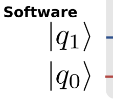
So for our two qubits the basis looks like
\[|\psi\rangle = |\hbox{qubit-1}\rangle \otimes |\hbox{qubit-0}\rangle =
\begin{pmatrix}
|0\rangle\otimes|0\rangle\\
|0\rangle\otimes|1\rangle\\
|1\rangle\otimes|0\rangle\\
|1\rangle\otimes|1\rangle\\
\end{pmatrix} =
\begin{pmatrix}
|00\rangle\\
|01\rangle\\
|10\rangle\\
|11\rangle\\
\end{pmatrix}\]
so that, e.g.
\[\begin{align}
|00\rangle &= \begin{pmatrix}
1\\
0\\
\end{pmatrix} \otimes \begin{pmatrix}
1\\
0\\
\end{pmatrix} = \begin{pmatrix}
1\\
0\\
0\\
0\\
\end{pmatrix},\\
|01\rangle &=
\begin{pmatrix}
1\\
0\\
\end{pmatrix} \otimes \begin{pmatrix}
0\\
1\\
\end{pmatrix} = \begin{pmatrix}
0\\
1\\
0\\
0\\
\end{pmatrix}, \mathrm{~etc.}
\end{align}\]
For two qubits, useful are the CNOT\(_{01}\) and CNOT\(_{10}\), where the first digit is the “control” qubit and the second is the “target” qubit. (Again, recall that in the O’Malley paper, we define qubit-1 as the “top” qubit, and qubit-0 as the “bottom” qubit, so if you change the qubit numbering the definitions will be swapped).
They can be defined as the sum of two tensor products:
\[\begin{align}
\mathrm{CNOT}_{10} &= (|0\rangle\langle 0| \otimes \mathbf{I}) + (|1\rangle\langle 1| \otimes {X}) = \begin{pmatrix}
1 & 0 & 0 & 0\\
0 & 1 & 0 & 0\\
0 & 0 & 0 & 1\\
0 & 0 & 1 & 0
\end{pmatrix}\\
\mathrm{CNOT}_{01} &= (\mathbf{I} \otimes |0\rangle\langle 0|) + (X \otimes |1\rangle\langle 1|) = \begin{pmatrix}
1 & 0 & 0 & 0\\
0 & 0 & 0 & 1\\
0 & 0 & 1 & 0\\
0 & 1 & 0 & 0
\end{pmatrix}\\
\end{align}\]
The SWAP gate does what you’d expect, swapping qubit 1 and qubit 0:
\[\mathrm{SWAP} = \begin{pmatrix}
1 & 0 & 0 & 0\\
0 & 0 & 1 & 0\\
0 & 1 & 0 & 0\\
0 & 0 & 0 & 1
\end{pmatrix}\\\]
Most other operations are just simple tensor products of the single qubit operations. Like if you want to apply a Pauli X gate to qubit 1 and a Pauli Y gate to qubit 0, it’s just \(X_1 \otimes Y_0\):
\[{X_1 \otimes Y_0} =
\begin{pmatrix}
0 & 1 \\
1 & 0 \\
\end{pmatrix}\otimes
\begin{pmatrix}
0 & -i \\
i & 0 \\
\end{pmatrix} =
\begin{pmatrix}
0 & 0 & 0 & -i\\
0 & 0 & i & 0\\
0 & -i & 0 & 0\\
i & 0 & 0 & 0\\
\end{pmatrix}\\\]
Okay, let’s get some of these coded up for later, and if we need any products, we know we can just np.kron them later as needed
from scipy.linalg import block_diag

# CNOTij, where i is control qubit and j is target qubit
CNOT10 = np.kron(P0,I) + np.kron(P1,Sx) # control -> q1, target -> q0
CNOT01 = np.kron(I,P0) + np.kron(Sx,P1) # control -> q0, target -> q1

SWAP   = block_diag(1,Sx,1)
Make that Hamiltonian!
Now we have our building blocks, we need to think about how to represent the Hamiltonian, which is usually in the fermion basis, in the basis of qubits. There are a few ways to do this, but the most common are the Jordan-Wigner (JW) transformation and the Bravyi-Kitaev (BK) transformation.
According to the O’Malley paper, using the BK-transformed Hamiltonian and exploiting some of the symmetry in the H\(_2\) molecule, the Hamiltonian can be represented by only two qubits. (Nice.) The Hamiltonian has five components:
\[\hat{H}_{\mathrm{BK}} = g_0 \mathbf{I} + g_1 Z_0 + g_2 Z_1 + g_3 Z_0Z_1 + g_4 Y_0Y_1 + g_5 X_0 X_1\]
It general, the coefficients \(g_i\) can be obtained from a cheap Hartree-Fock calculation.
So let’s build a Hamiltonian for the H\(_2\) molecule with a bond length of 0.75 A. We will also also add the nuclear repulsion energy nuclear_repulsion. The parameters we use can be found in Table 1 of the Appendix in the O’Malley paper, though for the nuclear repulsion energy you have to calculate yourself (I used Gaussian).
# See DOI: 10.1103/PhysRevX.6.031007
# Here, we use parameters given for H2 at R=0.75A
g0 = -0.4804
g1 = +0.3435
g2 = -0.4347
g3 = +0.5716
g4 = +0.0910
g5 = +0.0910

nuclear_repulsion = 0.7055696146
With all this, we can build the Hamiltonian, Hmol, explicitly in matrix form by taking tensor products, also known as Kronecker products (using np.kron), of the single-qubit matrix operators we built previously.
Hmol = (g0 * np.kron( I, I) + # g0 * I
        g1 * np.kron( I,Sz) + # g1 * Z0
        g2 * np.kron(Sz, I) + # g2 * Z1
        g3 * np.kron(Sz,Sz) + # g3 * Z0Z1
        g4 * np.kron(Sy,Sy) + # g4 * Y0Y1
        g5 * np.kron(Sx,Sx))  # g5 * X0X1
And let’s take a look at the Hamiltonian matrix:
    [[ 0.0000+0.j  0.0000+0.j  0.0000+0.j  0.0000+0.j]
     [ 0.0000+0.j -1.8302+0.j  0.1820+0.j  0.0000+0.j]
     [ 0.0000+0.j  0.1820+0.j -0.2738+0.j  0.0000+0.j]
     [ 0.0000+0.j  0.0000+0.j  0.0000+0.j  0.1824+0.j]]
Since we have the Hamiltonian in the computational basis, let’s just diagonalize it to get the energy (lowest eigenvalue). By adding the nuclear repulsion energy to the result we should get the same result as a Full Configuration Interaction (FCI) calculation.
electronic_energy = np.linalg.eigvalsh(Hmol)[0] # take the lowest value
print("Classical diagonalization: {:+2.8} Eh".format(electronic_energy + nuclear_repulsion))
print("Exact (from G16):          {:+2.8} Eh".format(-1.1457416808))
    Classical diagonalization: -1.1456295 Eh
    Exact (from G16):          -1.1457417 Eh
Considering that the Hamiltonian elements had a precision of 1E-04, this is very good agreement. However, this approach utilizes a classical algorithm to obtain the eigenvalues. We want to see if we can obtain the eigenvalues using a quantum circuit.
A first attempt at a quantum circuit
The usual input for quantum algorithms is to start in the \(\vert00\cdots\rangle\) state. This is represented by a zero vector, with the first element set to 1. Because our Hamiltonian for H\(_2\) only requires two qubits, we will start with the state \(\vert01\rangle\). To obtain this from \(\vert00\rangle\), we just need to act on the zeroth qubit with the Pauli X operator. This is the first step in the quantum circuit in the figure I showed above from the O’Malley paper. (They apply X\(_{\pi}\); same thing.)
# initial basis, put in |01> state with Sx operator on q0
psi0 = np.zeros((4,1))
psi0[0] = 1
psi0 = np.dot(np.kron(I,Sx),psi0)
print(psi0)
[[ 0.]
 [ 1.]
 [ 0.]
 [ 0.]]
We haven’t defined our VQE ansatz yet, but before we do, let’s write a function to return the expected value of the Hamiltonian Hmol given an ansatz, its parameter theta, and the initial state psi0. This ansatz will eventually be encoded by the quantum circuit.
def expected(theta,ansatz,Hmol,psi0):
    circuit = ansatz(theta[0])
    psi = np.dot(circuit,psi0)
    return np.real(np.dot(psi.conj().T,np.dot(Hmol,psi)))[0,0]
With the expectation value in hand, we now define an ansatz. In the O’Malley paper, they utilize the Unitary Coupled Cluster (UCC) ansatz, which in this case depends only on a single parameter \(\theta\):
\[U(\theta) = \mathrm{exp}\left(-i\theta X_0Y_1\right)\]
so that a parameterized wave function \(\vert\psi(\theta)\rangle\) for the ground state of H\(_2\) is given as
\[|\psi(\theta)\rangle = \mathrm{exp}\left(-i\theta X_0Y_1\right)|01\rangle\]
and \(X_0Y_1\) is the tensor product of the Pauli-X on qubit 0 and Pauli-Y on qubit 1.
Before thinking about how we might represent \(U(\theta)\) as a series of quantum gates, let’s plug it into the expression
\[E(\theta) = \frac{\langle \psi | U^{\dagger}(\theta)\hat{H}_{\mathrm{mol}}U(\theta)|\psi\rangle}{\langle \psi | U^{\dagger}(\theta)U(\theta)|\psi\rangle} = \langle \psi | U^{\dagger}(\theta)\hat{H}_{\mathrm{mol}}U(\theta)|\psi\rangle\]
(Note that as long as \(\psi\) is normalized and \(U\) is unitary, we can ignore the normalization \(\langle \psi \vert U^{\dagger}(\theta)U(\theta)\vert\psi\rangle\), since it always equals 1.)
Given the ansatz and the initial state psi0, we can minimize expected() using the classical optimizers in the scipy package. So straightforwardly plugging in and minimizing yields the lazy result:
from scipy.linalg import expm
from scipy.optimize import minimize

# our UCC ansatz, not yet represented in terms of quantum gates
ansatz = lambda theta: expm(-1j*np.array([theta])*np.kron(Sy,Sx))

# initial guess for theta
theta  = [0.0]
result = minimize(expected,theta,args=(ansatz,Hmol,psi0))
theta  = result.x[0]
val    = result.fun

print("Lazy VQE: ")
print("  [+] theta:  {:+2.8} deg".format(theta))
print("  [+] energy: {:+2.8} Eh".format(val + nuclear_repulsion))
Lazy VQE:
  [+] theta:  -0.11487186 deg
  [+] energy: -1.1456295 Eh
Which equals the result we got from diagonalization of the Hamiltonian. So we know that the UCC ansatz works! But we were lazy and didn’t bother to think about how the quantum computer would compute the exponential. So, how do we represent the UCC ansatz in terms of quantum gates acting on the initial qubit state?
A “real” quantum circuit
So before we saw the UCC ansatz works, but we cheated by keeping it as a matrix exponential. This is not a suitable form for a quantum computer. Let’s do better.
According to the O’Malley paper , we can represent \(U(\theta)\) for this problem as:
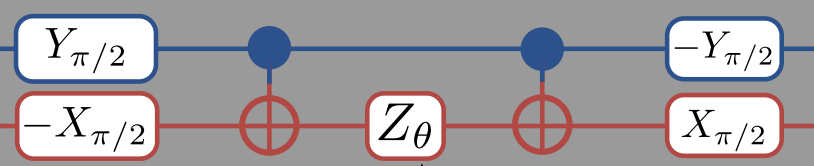
This means that we should change our ansatz to read
# read right-to-left (bottom-to-top?)

ansatz = lambda theta: (np.dot(np.dot(np.kron(-Ry(np.pi/2),Rx(np.pi/2)),
                        np.dot(CNOT10,
                        np.dot(np.kron(I,Rz(theta)),
                               CNOT10))),
                               np.kron(Ry(np.pi/2),-Rx(np.pi/2))))
Note that while you read the the circuit diagram left-to-right, when you read the matrix expression above it is better read right-to-left. The right-most matrices are applied to the state first, so that the first gates we apply are -R\(_x(\pi/2)\) to qubit-0 and R\(_y(\pi/2)\) to qubit-1. Also note that when we apply these two gates, it is simultaneous so the “total” gate is really -R\(_y(\pi/2) \otimes\)R\(_x(\pi/2)\).
theta  = [0.0]
result = minimize(expected,theta,args=(ansatz,Hmol,psi0))
theta  = result.x[0]
val    = result.fun

print("VQE: ")
print("  [+] theta:  {:+2.8} deg".format(theta))
print("  [+] energy: {:+2.8} Eh".format(val + nuclear_repulsion))
VQE:
  [+] theta:  +2.9118489 deg
  [+] energy: -1.1456295 Eh
Which is the correct answer! Since we can now compute the expectation value of our Hamiltonian using quantum gates, we can pass the computed energy to a classical optimizer, which gives new parameters for the quantum gates. When this process is repeated until convergence, we obtain the FCI ground state energy. Also, once we have the optimized wave function parameters, the ground state can be easily reconstructed for additional simulations, etc.
You might have noticed, though, that the above is still not sufficient for a quantum computer. The reason is that although we have represented our wave function with quantum gates, the measurement of the expectation value is still poorly defined as a physical operation. Even if you have prepared your qubits to represent a molecular wave function, measuring the expectation value of the Hamiltonian is not simply accomplished physically by applying a “Hamiltonian operation”.
An analogy: similar to classical computation, you might want a string, or float, or whatever as the “true” output of your function, but for the computer to compute it for you – it needs to ultimately be in binary. Same thing for the quantum computer. Our function should ultimately return the energy, but it needs to process this in terms of quantum bits.
A “real” measurement of the energy
All that is to say that we were cheating again. Experimentally, the “only” measurements we can make are those which probe the final quantum state of the qubits. What we need a way to connect measurements of qubits to an expression for the expectation value of the molecular electronic Hamiltonian.
Put another way, the problem stems back to our definition of the expected value:
def expected(theta,ansatz,Hmol,psi0):
    circuit = ansatz(theta[0])
    psi = np.dot(circuit,psi0)
    return np.real(np.dot(psi.conj().T,np.dot(Hmol,psi)))[0,0]
Simply dotting in Hmol with the wave function will not work, because physically we don’t have a measuring apparatus for “energy”. We can, however, measure the state of each qubit by measuring the spin (\(\hat{\mathrm{S}}_z\)) of each qubit. We need to reduce the Hamiltonian’s expected value into these types of “easy” projective measurements that can be done in the computational basis. These are sums of Pauli measurements.
Now in some respects, we are already halfway there. For a normalized wave function \(\vert\psi'\rangle\):
\[E = \langle \psi'|\hat{H}_\mathrm{mol}|\psi'\rangle\]
and using the definition of our H\(_2\) Hamiltonian in the computational basis we have:
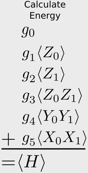
\[\begin{align} E &= \langle \psi'|g_0 \mathbf{I} + g_1 Z_0 + g_2 Z_1 + g_3 Z_0Z_1 + g_4 Y_0Y_1 + g_5 X_0 X_1|\psi'\rangle \\
&= g_0\langle \mathbf{I} \rangle + g_1\langle Z_0 \rangle + g_2 \langle Z_1 \rangle + g_3 \langle Z_0Z_1 \rangle + g_4 \langle Y_0Y_1 \rangle + g_5\langle X_0 X_1 \rangle \\
&= \sum_i g_i \langle \hat{O}_i \rangle
\end{align}\]
meaning that, given our wave function in the computational basis, if we can compute the expected value of the (products of) Pauli operators, we can relate this to the expected value of the Hamiltonian through the sum given above. This is given in that figure:
Let’s go a step further, though. It would be even better if we could relate the above expression to a single type of Pauli measurement, that is, measuring the spin of just one qubit. Then we don’t need to have multiple measurement apparatus.
Thankfully, there is a way to do this. The trick is to apply an additional unitary transformation at the end of the circuit so that, by measuring the spin of the top qubit, we can obtain any Pauli measurement. In our case, that means relating each of the the \(\langle \hat{O}_i\rangle\) quantities to the expected value of \(\langle Z_1 \otimes \mathbf{I}\rangle\) by some appropriate unitary operator. This is what is meant by the R\(_t\) gates in this part of the figure. The R\(_t\) are the unitaries we are talking about.
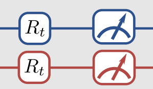
The little measuring gauge means we finally apply the measurement. Because we apply a particular form of the unitaries, we only need to measure the state of qubit-1 like we talked about above, but that’s not necessarily the only way to go about it.
You can find a table of some of these transformations here, but here are a few examples:
For example, the simplest case is if you want to measure \(Z_1 \otimes \mathbf{I}\). Then you don’t have to do anything:
\[\qquad Z_1 \otimes \mathbf{I} = (\mathbf{I} \otimes \mathbf{I})^{\dagger} \otimes (Z_1 \otimes \mathbf{I}) \otimes (\mathbf{I} \otimes \mathbf{I})\]
But if you want to measure \(Y_1 \otimes \mathbf{I}\), then
\[\qquad Y_1 \otimes \mathbf{I} = ({HS^{\dagger}} \otimes \mathbf{I})^{\dagger} \otimes (Z_1 \otimes \mathbf{I}) \otimes ({HS^{\dagger}} \otimes \mathbf{I})\]
For \(\mathbf{I} \otimes Z_0\), we have to apply the SWAP gate
\[\qquad \mathbf{I} \otimes Z_0 = (\mathrm{SWAP})^{\dagger} \otimes (Z_1 \otimes \mathbf{I}) \otimes (\mathrm{SWAP})\]
And as a final example, for \(X_1Z_0\), (caveat: we have different qubit ordering compared to the Microsoft documentation, so our CNOT\(_{10}\) vs CNOT\(_{01}\) definitions are swapped)
\[\qquad X_1 \otimes Z_0 = (\mathrm{CNOT}_{01}(H \otimes \mathbf{I}))^{\dagger} \otimes (Z_1 \otimes \mathbf{I}) \otimes (\mathrm{CNOT}_{01}(H \otimes \mathbf{I}))\]
Since you can think of these unitary transformations either acting on the operator, or acting on the state, the end result is that by applying the particular transformation and then measuring \(Z_1\) you can get any Pauli measurement you want.
It might be easier to see by example. Let’s see how this plays out for our Hamiltonian.
We will update the function expected() to projective_expected(), and remove the Hmol argument. In our case, this function will include the hard-coded representation of the Hamiltonian, in terms of measuring \(Z_1\).
def projective_expected(theta,ansatz,psi0):
    # this will depend on the hard-coded Hamiltonian + coefficients
    circuit = ansatz(theta[0])
    psi = np.dot(circuit,psi0)

    # for 2 qubits, assume we can only take Pauli Sz measurements (Sz \otimes I)
    # we just apply the right unitary for the desired Pauli measurement
    measureZ = lambda U: np.dot(np.conj(U).T,np.dot(np.kron(Sz,I),U))

    energy = 0.0

    # although the paper indexes the Hamiltonian left-to-right (0-to-1)
    # qubit-1 is always the top qubit for us, so the tensor pdt changes
    # e.g. compare with the "exact Hamiltonian" we explicitly diagonalized

    # <I1 I0>
    energy += g0 # it is a constant

    # <I1 Sz0>
    U = SWAP
    energy += g1*np.dot(psi.conj().T,np.dot(measureZ(U),psi))

    # <Sz1 I0>
    U = np.kron(I,I)
    energy += g2*np.dot(psi.conj().T,np.dot(measureZ(U),psi))

    # <Sz1 Sz0>
    U = CNOT01
    energy += g3*np.dot(psi.conj().T,np.dot(measureZ(U),psi))

    # <Sx1 Sx0>
    U = np.dot(CNOT01,np.kron(H,H))
    energy += g4*np.dot(psi.conj().T,np.dot(measureZ(U),psi))

    # <Sy1 Sy0>
    U = np.dot(CNOT01,np.kron(np.dot(H,S.conj().T),np.dot(H,S.conj().T)))
    energy += g5*np.dot(psi.conj().T,np.dot(measureZ(U),psi))

    return np.real(energy)[0,0]
With the expectation value now defined in terms of measuring the spin of the zero-th qubit, let’s carry out the VQE procedure:
theta  = [0.0]
result = minimize(projective_expected,theta,args=(ansatz,psi0))
theta  = result.x[0]
val    = result.fun

print("VQE: ")
print("  [+] theta:  {:+2.8} deg".format(theta))
print("  [+] energy: {:+2.8} Eh".format(val + nuclear_repulsion))
VQE:
  [+] theta:  +2.9118489 deg
  [+] energy: -1.1456295 Eh
Success! We get the same energy (and theta) as the previous VQE circuit, but now all measurements are related back to the result of measuring the spin of the qubit.
Appendix: All together now
Here’s all of the pieces together in one place
import numpy as np
from scipy.linalg import block_diag
from scipy.optimize import minimize

np.set_printoptions(precision=4,suppress=True)


# Pauli matrices
I  = np.array([[ 1, 0],
               [ 0, 1]])
Sx = np.array([[ 0, 1],
               [ 1, 0]])
Sy = np.array([[ 0,-1j],
               [1j, 0]])
Sz = np.array([[ 1, 0],
               [ 0,-1]])

# Hadamard matrix
H = (1/np.sqrt(2))*np.array([[ 1, 1],
                             [ 1,-1]])

# Phase matrix
S = np.array([[ 1, 0],
              [ 0,1j]])

# single qubit basis states |0> and |1>
q0 = np.array([[1],
               [0]])
q1 = np.array([[0],
               [1]])

# Projection matrices |0><0| and |1><1|
P0  = np.dot(q0,q0.conj().T)
P1  = np.dot(q1,q1.conj().T)


# Rotation matrices as a function of theta, e.g. Rx(theta), etc.
Rx = lambda theta : np.array([[    np.cos(theta/2),-1j*np.sin(theta/2)],
                              [-1j*np.sin(theta/2),    np.cos(theta/2)]])
Ry = lambda theta : np.array([[    np.cos(theta/2),   -np.sin(theta/2)],
                              [    np.sin(theta/2),    np.cos(theta/2)]])
Rz = lambda theta : np.array([[np.exp(-1j*theta/2),                0.0],
                              [                0.0, np.exp(1j*theta/2)]])

# CNOTij, where i is control qubit and j is target qubit
CNOT10 = np.kron(P0,I) + np.kron(P1,Sx) # control -> q1, target -> q0
CNOT01 = np.kron(I,P0) + np.kron(Sx,P1) # control -> q0, target -> q1

SWAP   = block_diag(1,Sx,1)

# See DOI: 10.1103/PhysRevX.6.031007
# Here, we use parameters given for H2 at R=0.75A
g0 = -0.4804
g1 = +0.3435
g2 = -0.4347
g3 = +0.5716
g4 = +0.0910
g5 = +0.0910

nuclear_repulsion = 0.7055696146

Hmol = (g0 * np.kron( I, I) + # g0 * I
        g1 * np.kron( I,Sz) + # g1 * Z0
        g2 * np.kron(Sz, I) + # g2 * Z1
        g3 * np.kron(Sz,Sz) + # g3 * Z0Z1
        g4 * np.kron(Sy,Sy) + # g4 * Y0Y1
        g5 * np.kron(Sx,Sx))  # g5 * X0X1

electronic_energy = np.linalg.eigvalsh(Hmol)[0] # take the lowest value
print("Classical diagonalization: {:+2.8} Eh".format(electronic_energy + nuclear_repulsion))
print("Exact (from G16):          {:+2.8} Eh".format(-1.1457416808))

# initial basis, put in |01> state with Sx operator on q0
psi0 = np.zeros((4,1))
psi0[0] = 1
psi0 = np.dot(np.kron(I,Sx),psi0)


# read right-to-left (bottom-to-top?)
ansatz = lambda theta: (np.dot(np.dot(np.kron(-Ry(np.pi/2),Rx(np.pi/2)),
                        np.dot(CNOT10,
                        np.dot(np.kron(I,Rz(theta)),
                               CNOT10))),
                               np.kron(Ry(np.pi/2),-Rx(np.pi/2))))

def projective_expected(theta,ansatz,psi0):
    # this will depend on the hard-coded Hamiltonian + coefficients
    circuit = ansatz(theta[0])
    psi = np.dot(circuit,psi0)

    # for 2 qubits, assume we can only take Pauli Sz measurements (Sz \otimes I)
    # we just apply the right unitary for the desired Pauli measurement
    measureZ = lambda U: np.dot(np.conj(U).T,np.dot(np.kron(Sz,I),U))

    energy = 0.0

    # although the paper indexes the hamiltonian left-to-right (0-to-1)
    # qubit-1 is always the top qubit for us, so the tensor pdt changes
    # e.g. compare with the "exact Hamiltonian" we explicitly diagonalized

    # <I1 I0>
    energy += g0 # it is a constant

    # <I1 Sz0>
    U = SWAP
    energy += g1*np.dot(psi.conj().T,np.dot(measureZ(U),psi))

    # <Sz1 I0>
    U = np.kron(I,I)
    energy += g2*np.dot(psi.conj().T,np.dot(measureZ(U),psi))

    # <Sz1 Sz0>
    U = CNOT01
    energy += g3*np.dot(psi.conj().T,np.dot(measureZ(U),psi))

    # <Sx1 Sx0>
    U = np.dot(CNOT01,np.kron(H,H))
    energy += g4*np.dot(psi.conj().T,np.dot(measureZ(U),psi))

    # <Sy1 Sy0>
    U = np.dot(CNOT01,np.kron(np.dot(H,S.conj().T),np.dot(H,S.conj().T)))
    energy += g5*np.dot(psi.conj().T,np.dot(measureZ(U),psi))

    return np.real(energy)[0,0]

theta  = [0.0]
result = minimize(projective_expected,theta,args=(ansatz,psi0))
theta  = result.x[0]
val    = result.fun

# check it works...
#assert np.allclose(val + nuclear_repulsion,-1.1456295)

print("VQE: ")
print("  [+] theta:  {:+2.8} deg".format(theta))
print("  [+] energy: {:+2.8} Eh".format(val + nuclear_repulsion))
Classical diagonalization: -1.1456295 Eh
Exact (from G16):          -1.1457417 Eh
VQE:
  [+] theta:  +2.9118489 deg
  [+] energy: -1.1456295 Eh
Most scientists are aware of the importance and significance of neural networks. Yet for many, neural networks remain mysterious and enigmatic.
Here, I want to show that neural networks are simply generalizations of something we scientists are perhaps more comfortable with: linear regression.
Regression models are models that find relationships among data. Linear regression models fit linear functions to data, like the \(y = mx + b\) equations we learned in algebra. If you have one variable, it’s single-variate linear regression; if you have more than one variable, it’s multi-variate linear regression.
One example of a linear regression model would be Charles’ Law which says that temperature and volume of a gas are proportional. By collecting temperatures and volumes of a gas, we can derive the proportionality constant between the two. For a multi-variable case, one example might be finding the relationship between the price of a house and its square footage and how many bedrooms it has.
It turns out we can write linear regression in terms of a graph like the one below. In this example we have two types of input data (features), \(x_1\) and \(x_2\). The function to be fit takes each of these data points, multiplies it by a weight \(w_1\) or \(w_2\) and adds them together. The \(b\) is the “bias”, which is analogous to the \(b\) in a linear equation \(y=mx+b\).
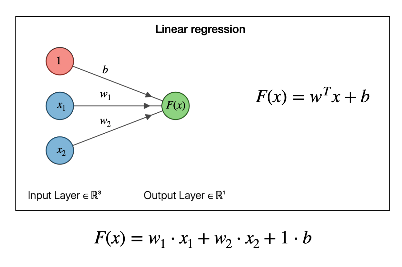
To make a model, we have to solve for the weights \(w\) and the bias \(b\). This can be done by many types of optimization algorithms (say, steepest descent or by pseudoinverse). Don’t worry about how the weights are obtained, just realize that that, one, we can obtain them and, two, once we have the weights and bias then we now have a functional relationship among our data.
So for example, if \(F(x)\) is housing price, and \(x_1\) is square footage and \(x_2\) is number of bedrooms, then we can predict the housing price given any house area and bedroom number via \(F(x) = w_1\cdot x_1 + w_2 \cdot x_2 + b\). So far so good.
Now we take things a bit further. The next step in our regression “evolution” is to pass the whole above linear regression model to a function. In the example below, we pass it to a sigmoid or logistic function \(\sigma(h)\). This is what logistic regression looks like as a graph:
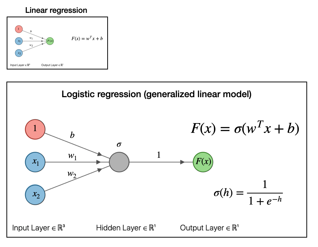
This is known as a “generalized linear model.” For our purposes, the exact function you pass the linear model into doesn’t matter so much. The important part is that we can make a generalized linear model by passing the linear model into a function. If you pass it into a sigmoid function, like we did above, you get a logistic regression model which can be useful for classification problems.
Like if I tell you the color and size of an animal, the logistic model can predict whether the animal is either a flamingo or an elephant.
So to recap, we started with a linear model, then by adding a function to the output, we got a generalized linear model. What’s the next step?
Glad you asked.
The next step with to take our linear model, pass it into a function (generalized linear model), then take that output and use it as an input for another linear model. If you do this, as depicted in the graph below, you will have obtained what is a called a shallow neural network.
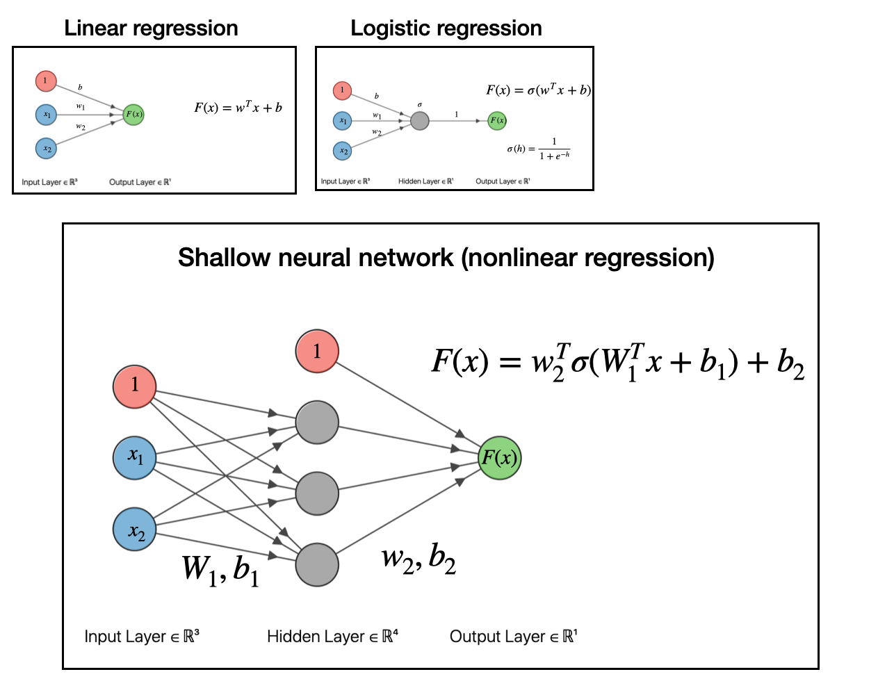
At this point, we have obtained a nonlinear regression model. That’s really all neural networks are: models for doing nonlinear regression.
At the end of the day all these models are doing the same thing, namely, finding relationships among data. Nonlinear regression allows you to find more complex relationships among the data. This doesn’t mean nonlinear regression is better, rather it is just a more flexible model. For many real-world problems, simpler linear regression is better! As long as it is suitable to handle your problem, it will be faster and easier to interpret.
So to recap, we went from linear regression, to logistic regression (a generalized linear model), to shallow neural network (nonlinear regression). The final step to get to deep neural networks is to pass the output of the shallow network into another function and make a linear model based off that output. This is depicted below:
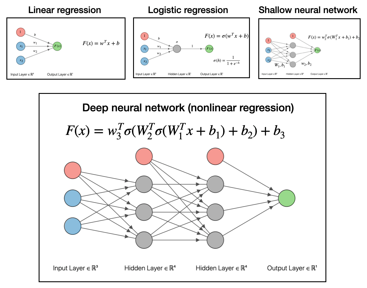
To reiterate, all these deep networks do is take data, make a linear model, transform with a function, then make another linear model with that output, transform that with a function, then make another linear model…and so on and so forth.
Data \(\to\) linear model \(\to\) function \(\to\) linear model \(\to\) function \(\to\) linear model…
It’s a series of nested functions that give you even more flexibility to handle strange nonlinear relationships among your data. And if that’s what your problem requires, that’s what it’s there for!
Obviously, modern developments of neural networks are far more complicated. I’m simplifying a lot of the details, but the general idea holds: neural networks are models to do nonlinear regression, and they are built up from linear models. They take one of the workhorses of scientific analysis, linear regression, and generalize it to handle complex, nonlinear relationships among data.
But as long as you keep in mind that it can be broken down to the pattern of passing the output of linear regression to a function, and then passing that output to another linear model, you can get pretty far.
Hope that helps!
I have a new review on (and titled) real-time time-dependent electronic structure theory out now, which has been one of my active research areas over the past five years or so. Like other electronic structure methods, real-time time-dependent (RT-TD) methods seeks to understand molecules through a quantum treatment of the motions of their electrons. What sets RT-TD theories and methods apart is that they explore how electrons evolve in time, especially as they respond to things like lasers, magnetic fields, X-rays, and so on. Real time methods look at molecular responses to these things explicitly in time, and gives an intuitive and dynamic view of how molecules behave under all sorts of experimental conditions. From this, we can predict and explain how certain molecules make better candidates for solar energy conversion, molecular electronics, or nanosensors, etc.
The truth is that there is a wealth of information that can be obtained by real-time time-dependent methods. Because of this, RT-TD methods are often criticized as inefficient and overkill for many predictive applications. In some cases this is true, for example when computing absorption spectra of small organic molecules (linear response methods are usually a better choice). However, to dismiss all RT-TD methods is a mistake, as the methods comprise a general technique for studying extremely complex phenomena. RT-TD methods allow for complete control over the number and strength of interacting external perturbations (multiple intense lasers, for example) in the study of molecular responses. In the review, we address many of these unique applications, ranging from non-equilibrium solvent dynamics to dynamic hyperpolarizability to the emerging real-time quantum electrodynamics (QED), where even the photon field is quantized.
The article was extremely fun to write, and I hope you find something useful and interesting in it. RT-TD comprises a broad field with extremely talented scientists working on its development. You can find the article here.
PDF version
The goal of all real-time electronic dynamics methods is to solve the
time-dependent Schrödinger equation (TDSE)
\[i\hbar \frac{\partial}{\partial t} \psi (t) = H(t) \psi(t)\]
where \(H(t)\) is the time-dependent Hamiltonian and \(\psi(t)\) is the
time-dependent wave function. The goal of the Magnus expansion is to
find a general solution for the time-dependent wave function in the case
where \(H\) is time-dependent, and, more crucially, when \(H\) does not
commute with itself at different times, e.g. when
\(\left[H(t_1),H(t_2)\right] \neq 0\). In the following we will follow
closely the notation of Blanes, et al..
First, for simplicity we redefine \(\tilde{H}(t) \equiv \frac{-i}{\hbar}H(t)\) and
introduce a scalar \(\lambda = 1\) as a bookkeeping device, so that
\[\begin{aligned}
\frac{\partial}{\partial t} \psi (t) &= \lambda \frac{-i}{\hbar} H(t) \psi(t) \\
&= \lambda \tilde{H}(t) \psi(t) \label{eq:tdse}\end{aligned}\]
At the heart of the Magnus expansion is the idea of solving the TDSE by
using the quantum propagator \(U(t,t_0)\) that connects wave functions at
different times, e.g. \(\psi(t) = U(t,t_0)\psi(t_0)\) Furthermore, the
Magnus expansion assumes that \(U(t,t_0)\) can be represented as an
exponential, \(U(t,t_0) = \text{exp} \left( \Omega(t,t_0) \right)\) This
yields the modified TDSE
\[\label{eq:modtdse}
\frac{\partial}{\partial t} U(t, t_0) = \lambda \tilde{H}(t) U(t,t_0); \quad U(t_0, t_0) = I\]
Now, for scalar \(H\) and \(U\), the above has a simple solution,
namely
\[U(t,t_0) = \text{exp} \left( \lambda \int\limits^{t}_{t_0} \tilde{H}(t') dt' \right)\]
However, if \(H\) and \(U\) are matrices this is not necessarily true. In
other words, for a given matrix \(A\) the following expression does not
necessarily hold:
\[\frac{\partial}{\partial t } \left( \text{exp}\left(A(t)\right) \right) = \left(\frac{\partial}{\partial t }A(t) \right)\text{exp}\left(A(t)\right) = \text{exp}\left(A(t)\right) \left(\frac{\partial}{\partial t } A(t) \right)\]
because the matrix \(A\) and its derivatives do not necessarily commute.
Instead, Magnus proved that in general \(\Omega (t, t_0)\)
satisfies
\[\frac{\partial}{\partial t} \left( \Omega(t,t_0) \right) = \lambda \tilde{H}(t) + \lambda \sum\limits_{k=1}^{\infty} (-1)^k \frac{B_k}{k!}\overbrace{[\Omega(t,t_0), [ \cdots[\Omega(t,t_0),}^{k-\text{times}} \tilde{H}(t)]] \cdots ]; \quad \Omega(t_0,t_0) = 0\]
where \(B_k\) are the Bernoulli numbers. This equation may be solved by
integration, and iterative substitution of \(\Omega(t,t_0)\). While it may
appear that we are worse off than when we started, collecting like
powers of \(\lambda\) (and setting \(\lambda = 1\)) allows us to obtain a
power-series expansion for \(\Omega(t,t_0)\),
\[\begin{aligned}
\label{eq:magnus}
\Omega(t,t_0) &= \int\limits_{t_0}^{t} \tilde{H}_1 dt_1 \\
&+ \frac{1}{2} \int\limits_{t_0}^{t} dt_1 \int\limits_{t_0}^{t_1} dt_2 \left[\tilde{H}_1,\tilde{H}_2\right] \\
&+ \frac{1}{6} \int\limits_{t_0}^{t} dt_1 \int\limits_{t_0}^{t_1} dt_2 \int\limits_{t_0}^{t_2} dt_3 \left( [\tilde{H}_1, [\tilde{H}_2, \tilde{H}_3]] + [\tilde{H}_3,[\tilde{H}_2,\tilde{H}_1]] \right) + \cdots\end{aligned}\]
This is the Magnus expansion, and here we have given up to the
third-order terms. We have also made the notational simplification that
\(\tilde{H}_k = \tilde{H}(t_k)\). This is the basis for nearly all
numerical methods to integrate the many-body TDSE in molecular physics.
Each subsequent order in the Magnus expansion is a correction that
accounts for the proper time-ordering of the Hamiltonian.
The Magnus expansion immediately suggests a route to
many numerical integrators. The simplest would be to approximate the
first term by
\[\int\limits_{t}^{t + \Delta t} \tilde{H}_1 dt_1 \approx \Delta t \tilde{H}(t)\]
leading to a forward-Euler-like time integrator of
\[\psi(t + \Delta t) = \text{exp}\left(\Delta t \tilde{H}(t)\right)\psi(t)\]
which we can re-write as
\[\psi(t_{k+1}) = \text{exp}\left(\Delta t \tilde{H}(t_{k})\right)\psi(t_{k})\]
where subscript \(k\) gives the node of the time-step stencil. This gives
a first-order method with error \(\mathcal{O}(\Delta t)\). A more accurate
second-order method can be constructed by approximating the first term
in the Magnus expansion by the midpoint rule, leading to an
\(\mathcal{O}({\Delta t}^2)\) time integrator
\[\psi(t_{k+1}) = \text{exp}\left(\Delta t \tilde{H}(t_{k+1/2})\right)\psi(t_{k})\]
Modifying the stencil to eliminate the need to evaluate the Hamiltonian
at fractional time steps (e.g. change time step to \(2 \Delta t\)) leads
to the modified midpoint unitary transformation (MMUT) method
\[\psi(t_{k+1}) = \text{exp}\left(2 \Delta t \tilde{H}(t_{k})\right)\psi(t_{k-1})\]
which is a leapfrog-type unitary integrator. Note that the midpoint
method assumes \(\tilde{H}\) is linear over its time interval, and the
higher order terms (containing the commutators) in this approximation go to zero. There are many other types of integrators
based off the Magnus expansion that can be found in the
literature. The key point for all of these
integrators is that they are symplectic, meaning they preserve
phase-space relationships. This has the practical effect of conserving
energy (within some error bound) in long-time dynamics, whereas
non-symplectic methods such as Runge-Kutta will experience energetic
“drift” over long times. A final note: in each of these schemes it is
necessary to evaluate the exponential of the Hamiltonian. In real-time
methods, this requires computing a matrix exponential. This is not a
trivial task, and, aside from the construction of the Hamiltonian
itself, is often the most expensive step in the numerical solution of
the TDSE. However, many elegant solutions to the construction of the
matrix exponential can be found in the literature.
References
Blanes, S., Casas, F., Oteo, J.A. and Ros, J., 2010. A pedagogical approach to the Magnus expansion. European Journal of Physics, 31(4), p.907.
Magnus, W., 1954. On the exponential solution of differential equations for a linear operator. Communications on pure and applied mathematics, 7(4), pp.649-673.