Variational Quantum Eigensolver (VQE) Example
Launch the interactive notebook: ![]()
Table of Contents
- Introduction
- Qubits, gates, and all that
- Make that Hamiltonian!
- A first attempt at a quantum circuit
- A “real” quantum circuit
- A “real” measurement of the energy
- Appendix: All together now
Introduction
The variational quantum eigensolver (VQE) is a hybrid classical-quantum algorithm that variationally determines the ground state energy of a Hamiltonian.
It’s quantum in the sense that the expectation value of the energy is computed via a quantum algorithm, but it is classical in the sense that the energy is minimized with a classical optimization algorithm.
From a molecular electronic structure perspective, it is equivalent to computing the Full Configuration Interaction (FCI) for a given basis.
Quantum computing can be a little unintuitive, so it helps to see a working example. Although we won’t actually do any “real” quantum computing, the methods can be understood from a linear algebra perspective. So that’s what we are going to try and do for the VQE.
The problem we want to tackle is to implement the VQE to compute the energy of molecular hydrogen (H\(_2\)) in a minimal basis. We will base this implementation off the really neat paper
O’Malley, Peter JJ, et al. “Scalable quantum simulation of molecular energies.” Physical Review X 6.3 (2016): 031007.
In the O’Malley paper, they implement the VQE on a real quantum computer to compute the potential energy surface of H\(_2\). The schematic we are going to follow can be seen below, and we are going to implement the “software”.
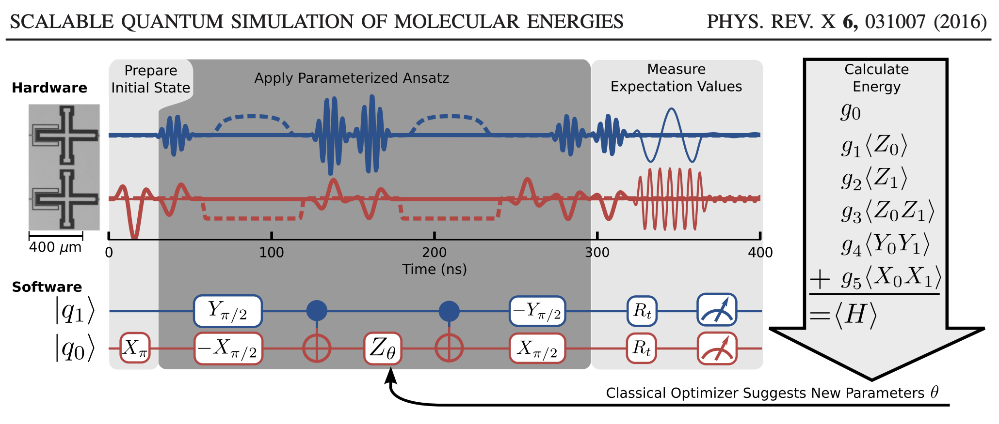
Here’s the big, overarching plan:
- Put the Hamiltonian in the computational (qubit) basis.
- Obtain a variational ansatz to parameterize the wave function.
- Represent this ansatz as a quantum circuit.
- Given this circuit, measure the expectation value of Hamiltonian (energy).
- Vary the circuit parameters until the energy is minimized.
We’ll look at these in turn, but first, let’s look at single qubit states and some common matrices used to operate on them. This will set the groundwork for building up our VQE procedure.
Qubits, gates, and all that
First, let’s define some of the common quantum operators, gates, and states we want to work with. For starters, here are the identity and Pauli spin matrices:
\[\mathbf{I} = \begin{pmatrix} 1 & 0 \\ 0 & 1 \end{pmatrix}\quad {X} = \begin{pmatrix} 0 & 1 \\ 1 & 0 \end{pmatrix}\quad {Y} = \begin{pmatrix} 0 & -i \\ i & 0 \end{pmatrix}\quad {Z} = \begin{pmatrix} 1 & 0 \\ 0 & -1 \end{pmatrix}\]Two other important gates are the Hadamard matrix and phase matrix:
\[{H} = \frac{1}{\sqrt{2}}\begin{pmatrix} 1 & 1 \\ 1 & -1 \end{pmatrix}\quad {S} = \begin{pmatrix} 1 & 0 \\ 0 & i \end{pmatrix}\]Since for a single qubit the two basis states are \(|\psi\rangle = \begin{pmatrix} |0\rangle\\ |1\rangle \end{pmatrix}, \quad \mathrm{meaning} \qquad |0\rangle = \begin{pmatrix} 1\\ 0 \end{pmatrix}\quad |1\rangle = \begin{pmatrix} 0\\ 1 \end{pmatrix}\)
we can define projection matrices, which are useful for defining, among other things, controlled gates (like CNOT, which we will see in a bit).
\[|0\rangle\langle 0| = \begin{pmatrix} 1 & 0 \\ 0 & 0 \end{pmatrix}\quad |1\rangle\langle 1| = \begin{pmatrix} 0 & 0\\ 0 & 1 \end{pmatrix}\]Also useful for single qubits, are the rotation matrices:
\[\begin{align} {R_x(\theta)} &= \begin{pmatrix} \mathrm{cos}(\theta/2) & -i\cdot\mathrm{sin}(\theta/2) \\ -i\cdot\mathrm{sin}(\theta/2) & \mathrm{cos}(\theta/2) \end{pmatrix}\\ {R_y(\theta)} &= \begin{pmatrix} \mathrm{cos}(\theta/2) & -\mathrm{sin}(\theta/2) \\ \mathrm{sin}(\theta/2) & \mathrm{cos}(\theta/2) \end{pmatrix}\\ {R_z(\theta)} &= \begin{pmatrix} \mathrm{exp}(-i\theta/2) & 0 \\ 0 & \mathrm{exp}(i\theta/2) \end{pmatrix} \end{align}\]So putting all these together for future use, we have:
import numpy as np
np.set_printoptions(precision=4,suppress=True)


# Pauli matrices
I  = np.array([[ 1, 0],
               [ 0, 1]])
Sx = np.array([[ 0, 1],
               [ 1, 0]])
Sy = np.array([[ 0,-1j],
               [1j, 0]])
Sz = np.array([[ 1, 0],
               [ 0,-1]])

# Hadamard matrix
H = (1/np.sqrt(2))*np.array([[ 1, 1],
                             [ 1,-1]])

# Phase matrix
S = np.array([[ 1, 0],
              [ 0,1j]])

# single qubit basis states |0> and |1>
q0 = np.array([[1],
               [0]])
q1 = np.array([[0],
               [1]])

# Projection matrices |0><0| and |1><1|
P0  = np.dot(q0,q0.conj().T)
P1  = np.dot(q1,q1.conj().T)


# Rotation matrices as a function of theta, e.g. Rx(theta), etc.
Rx = lambda theta : np.array([[    np.cos(theta/2),-1j*np.sin(theta/2)],
                              [-1j*np.sin(theta/2),    np.cos(theta/2)]])
Ry = lambda theta : np.array([[    np.cos(theta/2),   -np.sin(theta/2)],
                              [    np.sin(theta/2),    np.cos(theta/2)]])
Rz = lambda theta : np.array([[np.exp(-1j*theta/2),                0.0],
                              [                0.0, np.exp(1j*theta/2)]])
Next, using these single qubit operations, we can build up some common two-qubit states and operations. By and large, moving from single to multiple qubits just involves tensor products of single qubit states and gates. Note that we number our qubits from bottom to top in this example, so qubit-1 is on top and qubit-0 is on bottom; e.g. in the figure:
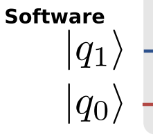
So for our two qubits the basis looks like
\[|\psi\rangle = |\hbox{qubit-1}\rangle \otimes |\hbox{qubit-0}\rangle = \begin{pmatrix} |0\rangle\otimes|0\rangle\\ |0\rangle\otimes|1\rangle\\ |1\rangle\otimes|0\rangle\\ |1\rangle\otimes|1\rangle\\ \end{pmatrix} = \begin{pmatrix} |00\rangle\\ |01\rangle\\ |10\rangle\\ |11\rangle\\ \end{pmatrix}\]so that, e.g.
\[\begin{align} |00\rangle &= \begin{pmatrix} 1\\ 0\\ \end{pmatrix} \otimes \begin{pmatrix} 1\\ 0\\ \end{pmatrix} = \begin{pmatrix} 1\\ 0\\ 0\\ 0\\ \end{pmatrix},\\ |01\rangle &= \begin{pmatrix} 1\\ 0\\ \end{pmatrix} \otimes \begin{pmatrix} 0\\ 1\\ \end{pmatrix} = \begin{pmatrix} 0\\ 1\\ 0\\ 0\\ \end{pmatrix}, \mathrm{~etc.} \end{align}\]For two qubits, useful are the CNOT\(_{01}\) and CNOT\(_{10}\), where the first digit is the “control” qubit and the second is the “target” qubit. (Again, recall that in the O’Malley paper, we define qubit-1 as the “top” qubit, and qubit-0 as the “bottom” qubit, so if you change the qubit numbering the definitions will be swapped).
They can be defined as the sum of two tensor products:
\[\begin{align} \mathrm{CNOT}_{10} &= (|0\rangle\langle 0| \otimes \mathbf{I}) + (|1\rangle\langle 1| \otimes {X}) = \begin{pmatrix} 1 & 0 & 0 & 0\\ 0 & 1 & 0 & 0\\ 0 & 0 & 0 & 1\\ 0 & 0 & 1 & 0 \end{pmatrix}\\ \mathrm{CNOT}_{01} &= (\mathbf{I} \otimes |0\rangle\langle 0|) + (X \otimes |1\rangle\langle 1|) = \begin{pmatrix} 1 & 0 & 0 & 0\\ 0 & 0 & 0 & 1\\ 0 & 0 & 1 & 0\\ 0 & 1 & 0 & 0 \end{pmatrix}\\ \end{align}\]The SWAP gate does what you’d expect, swapping qubit 1 and qubit 0:
\[\mathrm{SWAP} = \begin{pmatrix} 1 & 0 & 0 & 0\\ 0 & 0 & 1 & 0\\ 0 & 1 & 0 & 0\\ 0 & 0 & 0 & 1 \end{pmatrix}\\\]Most other operations are just simple tensor products of the single qubit operations. Like if you want to apply a Pauli X gate to qubit 1 and a Pauli Y gate to qubit 0, it’s just \(X_1 \otimes Y_0\):
\[{X_1 \otimes Y_0} = \begin{pmatrix} 0 & 1 \\ 1 & 0 \\ \end{pmatrix}\otimes \begin{pmatrix} 0 & -i \\ i & 0 \\ \end{pmatrix} = \begin{pmatrix} 0 & 0 & 0 & -i\\ 0 & 0 & i & 0\\ 0 & -i & 0 & 0\\ i & 0 & 0 & 0\\ \end{pmatrix}\\\]Okay, let’s get some of these coded up for later, and if we need any products, we know we can just np.kron them later as needed
from scipy.linalg import block_diag

# CNOTij, where i is control qubit and j is target qubit
CNOT10 = np.kron(P0,I) + np.kron(P1,Sx) # control -> q1, target -> q0
CNOT01 = np.kron(I,P0) + np.kron(Sx,P1) # control -> q0, target -> q1

SWAP   = block_diag(1,Sx,1)
Make that Hamiltonian!
Now we have our building blocks, we need to think about how to represent the Hamiltonian, which is usually in the fermion basis, in the basis of qubits. There are a few ways to do this, but the most common are the Jordan-Wigner (JW) transformation and the Bravyi-Kitaev (BK) transformation.
According to the O’Malley paper, using the BK-transformed Hamiltonian and exploiting some of the symmetry in the H\(_2\) molecule, the Hamiltonian can be represented by only two qubits. (Nice.) The Hamiltonian has five components:
\[\hat{H}_{\mathrm{BK}} = g_0 \mathbf{I} + g_1 Z_0 + g_2 Z_1 + g_3 Z_0Z_1 + g_4 Y_0Y_1 + g_5 X_0 X_1\]It general, the coefficients \(g_i\) can be obtained from a cheap Hartree-Fock calculation.
So let’s build a Hamiltonian for the H\(_2\) molecule with a bond length of 0.75 A. We will also also add the nuclear repulsion energy nuclear_repulsion. The parameters we use can be found in Table 1 of the Appendix in the O’Malley paper, though for the nuclear repulsion energy you have to calculate yourself (I used Gaussian).
# See DOI: 10.1103/PhysRevX.6.031007
# Here, we use parameters given for H2 at R=0.75A
g0 = -0.4804
g1 = +0.3435
g2 = -0.4347
g3 = +0.5716
g4 = +0.0910
g5 = +0.0910

nuclear_repulsion = 0.7055696146
With all this, we can build the Hamiltonian, Hmol, explicitly in matrix form by taking tensor products, also known as Kronecker products (using np.kron), of the single-qubit matrix operators we built previously.
Hmol = (g0 * np.kron( I, I) + # g0 * I
        g1 * np.kron( I,Sz) + # g1 * Z0
        g2 * np.kron(Sz, I) + # g2 * Z1
        g3 * np.kron(Sz,Sz) + # g3 * Z0Z1
        g4 * np.kron(Sy,Sy) + # g4 * Y0Y1
        g5 * np.kron(Sx,Sx))  # g5 * X0X1
And let’s take a look at the Hamiltonian matrix:
print(Hmol)
    [[ 0.0000+0.j  0.0000+0.j  0.0000+0.j  0.0000+0.j]
     [ 0.0000+0.j -1.8302+0.j  0.1820+0.j  0.0000+0.j]
     [ 0.0000+0.j  0.1820+0.j -0.2738+0.j  0.0000+0.j]
     [ 0.0000+0.j  0.0000+0.j  0.0000+0.j  0.1824+0.j]]
Since we have the Hamiltonian in the computational basis, let’s just diagonalize it to get the energy (lowest eigenvalue). By adding the nuclear repulsion energy to the result we should get the same result as a Full Configuration Interaction (FCI) calculation.
electronic_energy = np.linalg.eigvalsh(Hmol)[0] # take the lowest value
print("Classical diagonalization: {:+2.8} Eh".format(electronic_energy + nuclear_repulsion))
print("Exact (from G16):          {:+2.8} Eh".format(-1.1457416808))
    Classical diagonalization: -1.1456295 Eh
    Exact (from G16):          -1.1457417 Eh
Considering that the Hamiltonian elements had a precision of 1E-04, this is very good agreement. However, this approach utilizes a classical algorithm to obtain the eigenvalues. We want to see if we can obtain the eigenvalues using a quantum circuit.
A first attempt at a quantum circuit
The usual input for quantum algorithms is to start in the \(\vert00\cdots\rangle\) state. This is represented by a zero vector, with the first element set to 1. Because our Hamiltonian for H\(_2\) only requires two qubits, we will start with the state \(\vert01\rangle\). To obtain this from \(\vert00\rangle\), we just need to act on the zeroth qubit with the Pauli X operator. This is the first step in the quantum circuit in the figure I showed above from the O’Malley paper. (They apply X\(_{\pi}\); same thing.)
# initial basis, put in |01> state with Sx operator on q0
psi0 = np.zeros((4,1))
psi0[0] = 1
psi0 = np.dot(np.kron(I,Sx),psi0)
print(psi0)
[[ 0.]
 [ 1.]
 [ 0.]
 [ 0.]]
We haven’t defined our VQE ansatz yet, but before we do, let’s write a function to return the expected value of the Hamiltonian Hmol given an ansatz, its parameter theta, and the initial state psi0. This ansatz will eventually be encoded by the quantum circuit.
def expected(theta,ansatz,Hmol,psi0):
    circuit = ansatz(theta[0])
    psi = np.dot(circuit,psi0)
    return np.real(np.dot(psi.conj().T,np.dot(Hmol,psi)))[0,0]
With the expectation value in hand, we now define an ansatz. In the O’Malley paper, they utilize the Unitary Coupled Cluster (UCC) ansatz, which in this case depends only on a single parameter \(\theta\):
\[U(\theta) = \mathrm{exp}\left(-i\theta X_0Y_1\right)\]so that a parameterized wave function \(\vert\psi(\theta)\rangle\) for the ground state of H\(_2\) is given as
\[|\psi(\theta)\rangle = \mathrm{exp}\left(-i\theta X_0Y_1\right)|01\rangle\]and \(X_0Y_1\) is the tensor product of the Pauli-X on qubit 0 and Pauli-Y on qubit 1.
Before thinking about how we might represent \(U(\theta)\) as a series of quantum gates, let’s plug it into the expression
\[E(\theta) = \frac{\langle \psi | U^{\dagger}(\theta)\hat{H}_{\mathrm{mol}}U(\theta)|\psi\rangle}{\langle \psi | U^{\dagger}(\theta)U(\theta)|\psi\rangle} = \langle \psi | U^{\dagger}(\theta)\hat{H}_{\mathrm{mol}}U(\theta)|\psi\rangle\](Note that as long as \(\psi\) is normalized and \(U\) is unitary, we can ignore the normalization \(\langle \psi \vert U^{\dagger}(\theta)U(\theta)\vert\psi\rangle\), since it always equals 1.)
Given the ansatz and the initial state psi0, we can minimize expected() using the classical optimizers in the scipy package. So straightforwardly plugging in and minimizing yields the lazy result:
from scipy.linalg import expm
from scipy.optimize import minimize

# our UCC ansatz, not yet represented in terms of quantum gates
ansatz = lambda theta: expm(-1j*np.array([theta])*np.kron(Sy,Sx))

# initial guess for theta
theta  = [0.0]
result = minimize(expected,theta,args=(ansatz,Hmol,psi0))
theta  = result.x[0]
val    = result.fun

print("Lazy VQE: ")
print("  [+] theta:  {:+2.8} deg".format(theta))
print("  [+] energy: {:+2.8} Eh".format(val + nuclear_repulsion))
Lazy VQE:
  [+] theta:  -0.11487186 deg
  [+] energy: -1.1456295 Eh
Which equals the result we got from diagonalization of the Hamiltonian. So we know that the UCC ansatz works! But we were lazy and didn’t bother to think about how the quantum computer would compute the exponential. So, how do we represent the UCC ansatz in terms of quantum gates acting on the initial qubit state?
A “real” quantum circuit
So before we saw the UCC ansatz works, but we cheated by keeping it as a matrix exponential. This is not a suitable form for a quantum computer. Let’s do better.
According to the O’Malley paper , we can represent \(U(\theta)\) for this problem as:
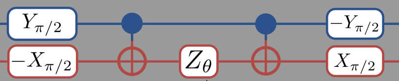
This means that we should change our ansatz to read
# read right-to-left (bottom-to-top?)

ansatz = lambda theta: (np.dot(np.dot(np.kron(-Ry(np.pi/2),Rx(np.pi/2)),
                        np.dot(CNOT10,
                        np.dot(np.kron(I,Rz(theta)),
                               CNOT10))),
                               np.kron(Ry(np.pi/2),-Rx(np.pi/2))))
Note that while you read the the circuit diagram left-to-right, when you read the matrix expression above it is better read right-to-left. The right-most matrices are applied to the state first, so that the first gates we apply are -R\(_x(\pi/2)\) to qubit-0 and R\(_y(\pi/2)\) to qubit-1. Also note that when we apply these two gates, it is simultaneous so the “total” gate is really -R\(_y(\pi/2) \otimes\)R\(_x(\pi/2)\).
theta  = [0.0]
result = minimize(expected,theta,args=(ansatz,Hmol,psi0))
theta  = result.x[0]
val    = result.fun

print("VQE: ")
print("  [+] theta:  {:+2.8} deg".format(theta))
print("  [+] energy: {:+2.8} Eh".format(val + nuclear_repulsion))
VQE:
  [+] theta:  +2.9118489 deg
  [+] energy: -1.1456295 Eh
Which is the correct answer! Since we can now compute the expectation value of our Hamiltonian using quantum gates, we can pass the computed energy to a classical optimizer, which gives new parameters for the quantum gates. When this process is repeated until convergence, we obtain the FCI ground state energy. Also, once we have the optimized wave function parameters, the ground state can be easily reconstructed for additional simulations, etc.
You might have noticed, though, that the above is still not sufficient for a quantum computer. The reason is that although we have represented our wave function with quantum gates, the measurement of the expectation value is still poorly defined as a physical operation. Even if you have prepared your qubits to represent a molecular wave function, measuring the expectation value of the Hamiltonian is not simply accomplished physically by applying a “Hamiltonian operation”.
An analogy: similar to classical computation, you might want a string, or float, or whatever as the “true” output of your function, but for the computer to compute it for you – it needs to ultimately be in binary. Same thing for the quantum computer. Our function should ultimately return the energy, but it needs to process this in terms of quantum bits.
A “real” measurement of the energy
All that is to say that we were cheating again. Experimentally, the “only” measurements we can make are those which probe the final quantum state of the qubits. What we need a way to connect measurements of qubits to an expression for the expectation value of the molecular electronic Hamiltonian.
Put another way, the problem stems back to our definition of the expected value:
def expected(theta,ansatz,Hmol,psi0):
    circuit = ansatz(theta[0])
    psi = np.dot(circuit,psi0)
    return np.real(np.dot(psi.conj().T,np.dot(Hmol,psi)))[0,0]
Simply dotting in Hmol with the wave function will not work, because physically we don’t have a measuring apparatus for “energy”. We can, however, measure the state of each qubit by measuring the spin (\(\hat{\mathrm{S}}_z\)) of each qubit. We need to reduce the Hamiltonian’s expected value into these types of “easy” projective measurements that can be done in the computational basis. These are sums of Pauli measurements.
Now in some respects, we are already halfway there. For a normalized wave function \(\vert\psi'\rangle\):
\[E = \langle \psi'|\hat{H}_\mathrm{mol}|\psi'\rangle\]and using the definition of our H\(_2\) Hamiltonian in the computational basis we have:
\[\begin{align} E &= \langle \psi'|g_0 \mathbf{I} + g_1 Z_0 + g_2 Z_1 + g_3 Z_0Z_1 + g_4 Y_0Y_1 + g_5 X_0 X_1|\psi'\rangle \\ &= g_0\langle \mathbf{I} \rangle + g_1\langle Z_0 \rangle + g_2 \langle Z_1 \rangle + g_3 \langle Z_0Z_1 \rangle + g_4 \langle Y_0Y_1 \rangle + g_5\langle X_0 X_1 \rangle \\ &= \sum_i g_i \langle \hat{O}_i \rangle \end{align}\]meaning that, given our wave function in the computational basis, if we can compute the expected value of the (products of) Pauli operators, we can relate this to the expected value of the Hamiltonian through the sum given above. This is given in that figure:
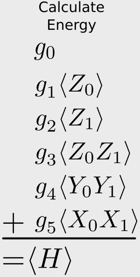
Let’s go a step further, though. It would be even better if we could relate the above expression to a single type of Pauli measurement, that is, measuring the spin of just one qubit. Then we don’t need to have multiple measurement apparatus.
Thankfully, there is a way to do this. The trick is to apply an additional unitary transformation at the end of the circuit so that, by measuring the spin of the top qubit, we can obtain any Pauli measurement. In our case, that means relating each of the the \(\langle \hat{O}_i\rangle\) quantities to the expected value of \(\langle Z_1 \otimes \mathbf{I}\rangle\) by some appropriate unitary operator. This is what is meant by the R\(_t\) gates in this part of the figure. The R\(_t\) are the unitaries we are talking about.
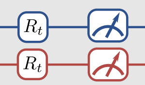
The little measuring gauge means we finally apply the measurement. Because we apply a particular form of the unitaries, we only need to measure the state of qubit-1 like we talked about above, but that’s not necessarily the only way to go about it.
You can find a table of some of these transformations here, but here are a few examples:
For example, the simplest case is if you want to measure \(Z_1 \otimes \mathbf{I}\). Then you don’t have to do anything:
\[\qquad Z_1 \otimes \mathbf{I} = (\mathbf{I} \otimes \mathbf{I})^{\dagger} \otimes (Z_1 \otimes \mathbf{I}) \otimes (\mathbf{I} \otimes \mathbf{I})\]But if you want to measure \(Y_1 \otimes \mathbf{I}\), then
\[\qquad Y_1 \otimes \mathbf{I} = ({HS^{\dagger}} \otimes \mathbf{I})^{\dagger} \otimes (Z_1 \otimes \mathbf{I}) \otimes ({HS^{\dagger}} \otimes \mathbf{I})\]For \(\mathbf{I} \otimes Z_0\), we have to apply the SWAP gate
\[\qquad \mathbf{I} \otimes Z_0 = (\mathrm{SWAP})^{\dagger} \otimes (Z_1 \otimes \mathbf{I}) \otimes (\mathrm{SWAP})\]And as a final example, for \(X_1Z_0\), (caveat: we have different qubit ordering compared to the Microsoft documentation, so our CNOT\(_{10}\) vs CNOT\(_{01}\) definitions are swapped)
\[\qquad X_1 \otimes Z_0 = (\mathrm{CNOT}_{01}(H \otimes \mathbf{I}))^{\dagger} \otimes (Z_1 \otimes \mathbf{I}) \otimes (\mathrm{CNOT}_{01}(H \otimes \mathbf{I}))\]Since you can think of these unitary transformations either acting on the operator, or acting on the state, the end result is that by applying the particular transformation and then measuring \(Z_1\) you can get any Pauli measurement you want.
It might be easier to see by example. Let’s see how this plays out for our Hamiltonian.
We will update the function expected() to projective_expected(), and remove the Hmol argument. In our case, this function will include the hard-coded representation of the Hamiltonian, in terms of measuring \(Z_1\).
def projective_expected(theta,ansatz,psi0):
    # this will depend on the hard-coded Hamiltonian + coefficients
    circuit = ansatz(theta[0])
    psi = np.dot(circuit,psi0)

    # for 2 qubits, assume we can only take Pauli Sz measurements (Sz \otimes I)
    # we just apply the right unitary for the desired Pauli measurement
    measureZ = lambda U: np.dot(np.conj(U).T,np.dot(np.kron(Sz,I),U))

    energy = 0.0

    # although the paper indexes the Hamiltonian left-to-right (0-to-1)
    # qubit-1 is always the top qubit for us, so the tensor pdt changes
    # e.g. compare with the "exact Hamiltonian" we explicitly diagonalized

    # <I1 I0>
    energy += g0 # it is a constant

    # <I1 Sz0>
    U = SWAP
    energy += g1*np.dot(psi.conj().T,np.dot(measureZ(U),psi))

    # <Sz1 I0>
    U = np.kron(I,I)
    energy += g2*np.dot(psi.conj().T,np.dot(measureZ(U),psi))

    # <Sz1 Sz0>
    U = CNOT01
    energy += g3*np.dot(psi.conj().T,np.dot(measureZ(U),psi))

    # <Sx1 Sx0>
    U = np.dot(CNOT01,np.kron(H,H))
    energy += g4*np.dot(psi.conj().T,np.dot(measureZ(U),psi))

    # <Sy1 Sy0>
    U = np.dot(CNOT01,np.kron(np.dot(H,S.conj().T),np.dot(H,S.conj().T)))
    energy += g5*np.dot(psi.conj().T,np.dot(measureZ(U),psi))

    return np.real(energy)[0,0]
With the expectation value now defined in terms of measuring the spin of the zero-th qubit, let’s carry out the VQE procedure:
theta  = [0.0]
result = minimize(projective_expected,theta,args=(ansatz,psi0))
theta  = result.x[0]
val    = result.fun

print("VQE: ")
print("  [+] theta:  {:+2.8} deg".format(theta))
print("  [+] energy: {:+2.8} Eh".format(val + nuclear_repulsion))
VQE:
  [+] theta:  +2.9118489 deg
  [+] energy: -1.1456295 Eh
Success! We get the same energy (and theta) as the previous VQE circuit, but now all measurements are related back to the result of measuring the spin of the qubit.
Appendix: All together now
Here’s all of the pieces together in one place
import numpy as np
from scipy.linalg import block_diag
from scipy.optimize import minimize

np.set_printoptions(precision=4,suppress=True)


# Pauli matrices
I  = np.array([[ 1, 0],
               [ 0, 1]])
Sx = np.array([[ 0, 1],
               [ 1, 0]])
Sy = np.array([[ 0,-1j],
               [1j, 0]])
Sz = np.array([[ 1, 0],
               [ 0,-1]])

# Hadamard matrix
H = (1/np.sqrt(2))*np.array([[ 1, 1],
                             [ 1,-1]])

# Phase matrix
S = np.array([[ 1, 0],
              [ 0,1j]])

# single qubit basis states |0> and |1>
q0 = np.array([[1],
               [0]])
q1 = np.array([[0],
               [1]])

# Projection matrices |0><0| and |1><1|
P0  = np.dot(q0,q0.conj().T)
P1  = np.dot(q1,q1.conj().T)


# Rotation matrices as a function of theta, e.g. Rx(theta), etc.
Rx = lambda theta : np.array([[    np.cos(theta/2),-1j*np.sin(theta/2)],
                              [-1j*np.sin(theta/2),    np.cos(theta/2)]])
Ry = lambda theta : np.array([[    np.cos(theta/2),   -np.sin(theta/2)],
                              [    np.sin(theta/2),    np.cos(theta/2)]])
Rz = lambda theta : np.array([[np.exp(-1j*theta/2),                0.0],
                              [                0.0, np.exp(1j*theta/2)]])

# CNOTij, where i is control qubit and j is target qubit
CNOT10 = np.kron(P0,I) + np.kron(P1,Sx) # control -> q1, target -> q0
CNOT01 = np.kron(I,P0) + np.kron(Sx,P1) # control -> q0, target -> q1

SWAP   = block_diag(1,Sx,1)

# See DOI: 10.1103/PhysRevX.6.031007
# Here, we use parameters given for H2 at R=0.75A
g0 = -0.4804
g1 = +0.3435
g2 = -0.4347
g3 = +0.5716
g4 = +0.0910
g5 = +0.0910

nuclear_repulsion = 0.7055696146

Hmol = (g0 * np.kron( I, I) + # g0 * I
        g1 * np.kron( I,Sz) + # g1 * Z0
        g2 * np.kron(Sz, I) + # g2 * Z1
        g3 * np.kron(Sz,Sz) + # g3 * Z0Z1
        g4 * np.kron(Sy,Sy) + # g4 * Y0Y1
        g5 * np.kron(Sx,Sx))  # g5 * X0X1

electronic_energy = np.linalg.eigvalsh(Hmol)[0] # take the lowest value
print("Classical diagonalization: {:+2.8} Eh".format(electronic_energy + nuclear_repulsion))
print("Exact (from G16):          {:+2.8} Eh".format(-1.1457416808))

# initial basis, put in |01> state with Sx operator on q0
psi0 = np.zeros((4,1))
psi0[0] = 1
psi0 = np.dot(np.kron(I,Sx),psi0)


# read right-to-left (bottom-to-top?)
ansatz = lambda theta: (np.dot(np.dot(np.kron(-Ry(np.pi/2),Rx(np.pi/2)),
                        np.dot(CNOT10,
                        np.dot(np.kron(I,Rz(theta)),
                               CNOT10))),
                               np.kron(Ry(np.pi/2),-Rx(np.pi/2))))

def projective_expected(theta,ansatz,psi0):
    # this will depend on the hard-coded Hamiltonian + coefficients
    circuit = ansatz(theta[0])
    psi = np.dot(circuit,psi0)

    # for 2 qubits, assume we can only take Pauli Sz measurements (Sz \otimes I)
    # we just apply the right unitary for the desired Pauli measurement
    measureZ = lambda U: np.dot(np.conj(U).T,np.dot(np.kron(Sz,I),U))

    energy = 0.0

    # although the paper indexes the hamiltonian left-to-right (0-to-1)
    # qubit-1 is always the top qubit for us, so the tensor pdt changes
    # e.g. compare with the "exact Hamiltonian" we explicitly diagonalized

    # <I1 I0>
    energy += g0 # it is a constant

    # <I1 Sz0>
    U = SWAP
    energy += g1*np.dot(psi.conj().T,np.dot(measureZ(U),psi))

    # <Sz1 I0>
    U = np.kron(I,I)
    energy += g2*np.dot(psi.conj().T,np.dot(measureZ(U),psi))

    # <Sz1 Sz0>
    U = CNOT01
    energy += g3*np.dot(psi.conj().T,np.dot(measureZ(U),psi))

    # <Sx1 Sx0>
    U = np.dot(CNOT01,np.kron(H,H))
    energy += g4*np.dot(psi.conj().T,np.dot(measureZ(U),psi))

    # <Sy1 Sy0>
    U = np.dot(CNOT01,np.kron(np.dot(H,S.conj().T),np.dot(H,S.conj().T)))
    energy += g5*np.dot(psi.conj().T,np.dot(measureZ(U),psi))

    return np.real(energy)[0,0]

theta  = [0.0]
result = minimize(projective_expected,theta,args=(ansatz,psi0))
theta  = result.x[0]
val    = result.fun

# check it works...
#assert np.allclose(val + nuclear_repulsion,-1.1456295)

print("VQE: ")
print("  [+] theta:  {:+2.8} deg".format(theta))
print("  [+] energy: {:+2.8} Eh".format(val + nuclear_repulsion))
Classical diagonalization: -1.1456295 Eh
Exact (from G16):          -1.1457417 Eh
VQE:
  [+] theta:  +2.9118489 deg
  [+] energy: -1.1456295 Eh