Neural Networks by Analogy with Linear Regression
Most scientists are aware of the importance and significance of neural networks. Yet for many, neural networks remain mysterious and enigmatic.
Here, I want to show that neural networks are simply generalizations of something we scientists are perhaps more comfortable with: linear regression.
Regression models are models that find relationships among data. Linear regression models fit linear functions to data, like the \(y = mx + b\) equations we learned in algebra. If you have one variable, it’s single-variate linear regression; if you have more than one variable, it’s multi-variate linear regression.
One example of a linear regression model would be Charles’ Law which says that temperature and volume of a gas are proportional. By collecting temperatures and volumes of a gas, we can derive the proportionality constant between the two. For a multi-variable case, one example might be finding the relationship between the price of a house and its square footage and how many bedrooms it has.
It turns out we can write linear regression in terms of a graph like the one below. In this example we have two types of input data (features), \(x_1\) and \(x_2\). The function to be fit takes each of these data points, multiplies it by a weight \(w_1\) or \(w_2\) and adds them together. The \(b\) is the “bias”, which is analogous to the \(b\) in a linear equation \(y=mx+b\).
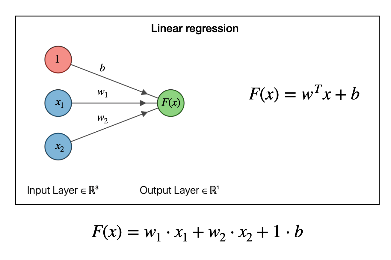
To make a model, we have to solve for the weights \(w\) and the bias \(b\). This can be done by many types of optimization algorithms (say, steepest descent or by pseudoinverse). Don’t worry about how the weights are obtained, just realize that that, one, we can obtain them and, two, once we have the weights and bias then we now have a functional relationship among our data.
So for example, if \(F(x)\) is housing price, and \(x_1\) is square footage and \(x_2\) is number of bedrooms, then we can predict the housing price given any house area and bedroom number via \(F(x) = w_1\cdot x_1 + w_2 \cdot x_2 + b\). So far so good.
Now we take things a bit further. The next step in our regression “evolution” is to pass the whole above linear regression model to a function. In the example below, we pass it to a sigmoid or logistic function \(\sigma(h)\). This is what logistic regression looks like as a graph:
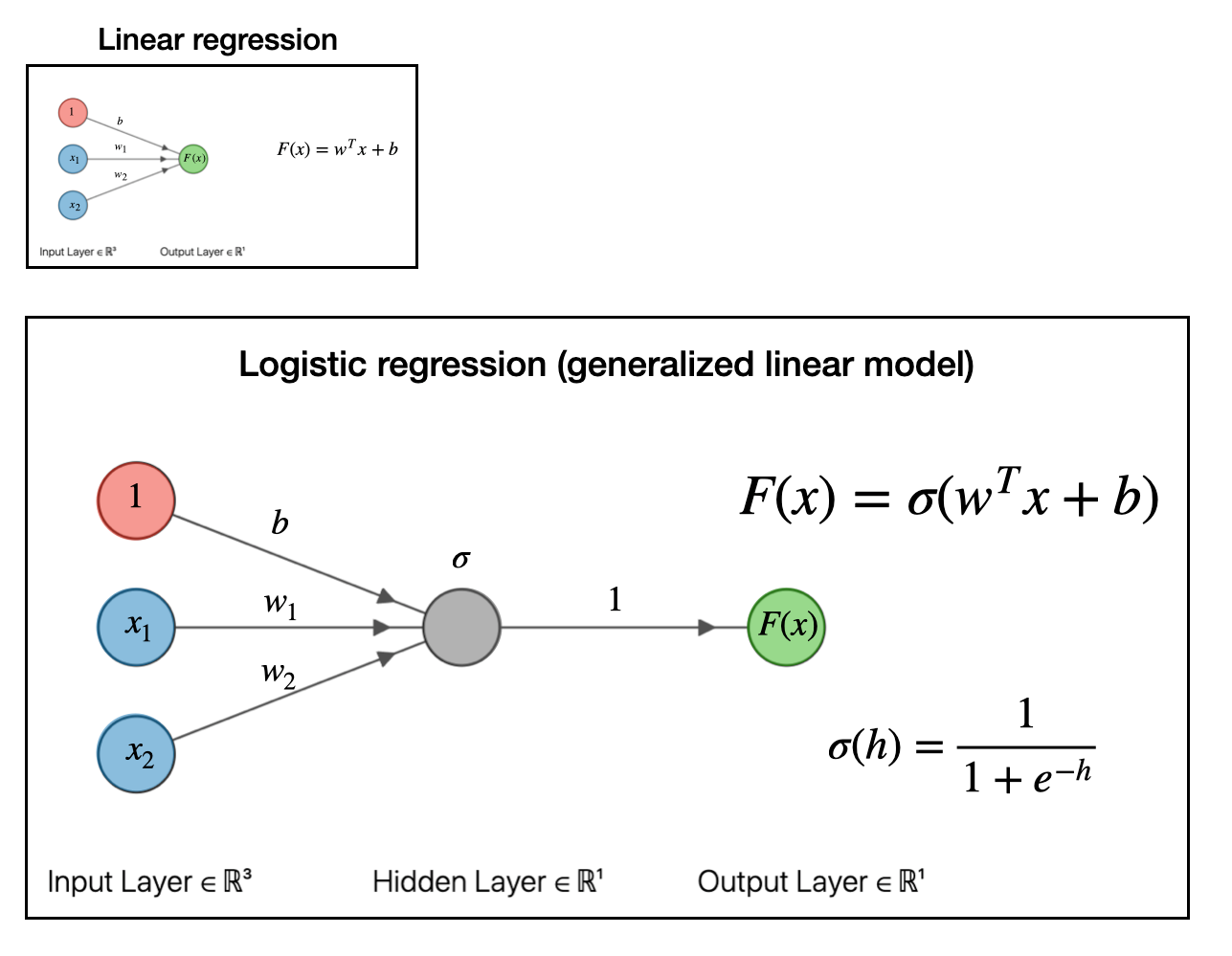
This is known as a “generalized linear model.” For our purposes, the exact function you pass the linear model into doesn’t matter so much. The important part is that we can make a generalized linear model by passing the linear model into a function. If you pass it into a sigmoid function, like we did above, you get a logistic regression model which can be useful for classification problems.
Like if I tell you the color and size of an animal, the logistic model can predict whether the animal is either a flamingo or an elephant.
So to recap, we started with a linear model, then by adding a function to the output, we got a generalized linear model. What’s the next step?
Glad you asked.
The next step with to take our linear model, pass it into a function (generalized linear model), then take that output and use it as an input for another linear model. If you do this, as depicted in the graph below, you will have obtained what is a called a shallow neural network.
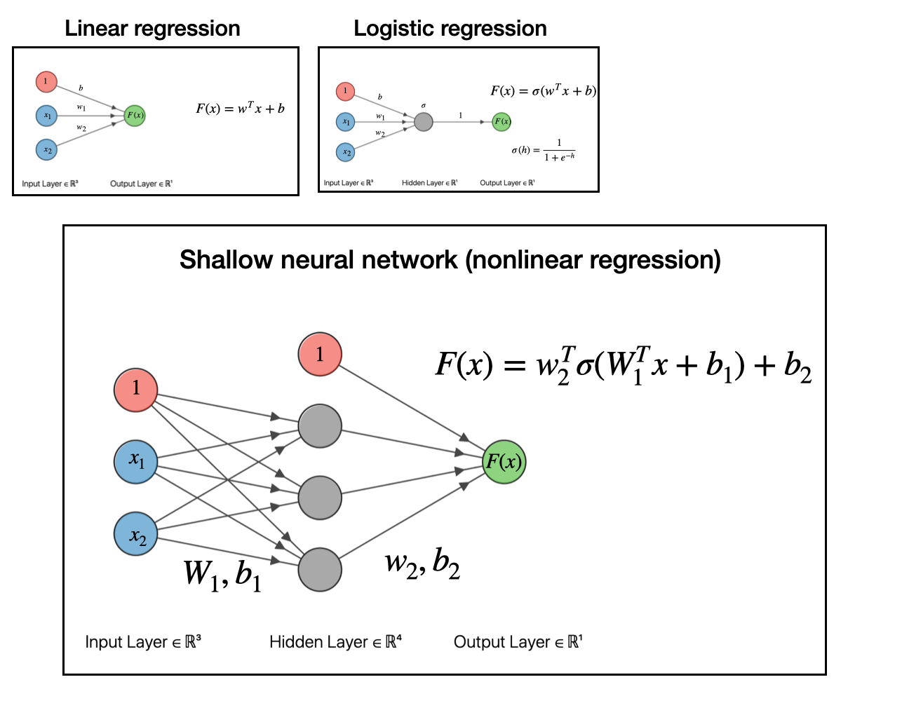
At this point, we have obtained a nonlinear regression model. That’s really all neural networks are: models for doing nonlinear regression.
At the end of the day all these models are doing the same thing, namely, finding relationships among data. Nonlinear regression allows you to find more complex relationships among the data. This doesn’t mean nonlinear regression is better, rather it is just a more flexible model. For many real-world problems, simpler linear regression is better! As long as it is suitable to handle your problem, it will be faster and easier to interpret.
So to recap, we went from linear regression, to logistic regression (a generalized linear model), to shallow neural network (nonlinear regression). The final step to get to deep neural networks is to pass the output of the shallow network into another function and make a linear model based off that output. This is depicted below:
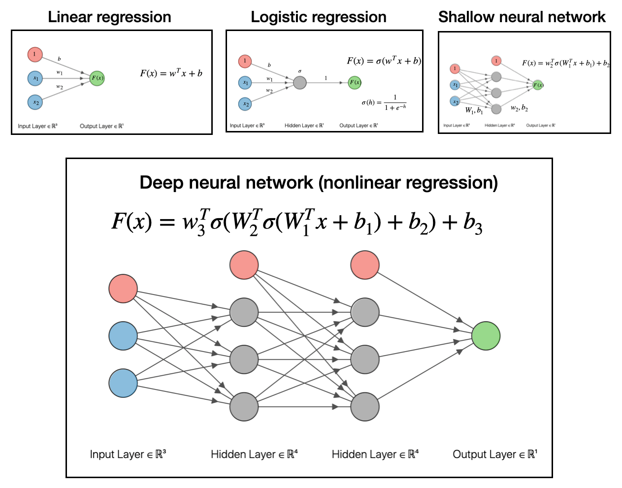
To reiterate, all these deep networks do is take data, make a linear model, transform with a function, then make another linear model with that output, transform that with a function, then make another linear model…and so on and so forth.
Data \(\to\) linear model \(\to\) function \(\to\) linear model \(\to\) function \(\to\) linear model…
It’s a series of nested functions that give you even more flexibility to handle strange nonlinear relationships among your data. And if that’s what your problem requires, that’s what it’s there for!
Obviously, modern developments of neural networks are far more complicated. I’m simplifying a lot of the details, but the general idea holds: neural networks are models to do nonlinear regression, and they are built up from linear models. They take one of the workhorses of scientific analysis, linear regression, and generalize it to handle complex, nonlinear relationships among data.
But as long as you keep in mind that it can be broken down to the pattern of passing the output of linear regression to a function, and then passing that output to another linear model, you can get pretty far.
Hope that helps!