Maximum Entropy Distributions

I think the method of maximum entropy to obtain probability distributions is so cool. You take a few knowns or constraints, and then maximize information entropy subject to these conditions and voila! you have a unique probability distribution. The cool thing is that these maximum entropy distributions are quite common, so this is a neat way of re-deriving many of the distibutions we encounter day-to-day. For me that alone is worth the cost of entry. But from an information-theoretic perspective, these will be the least biased prior distributions (we maximize our ignorance) so subsequent experiments a la Bayes’ theorem will maximize the information gained. Moreover, many physical patterns found in nature tend toward maximum entropy probability distributions. So even as a way to understand the world, maximum entropy is a very useful and deep tool.

Here are some common probability distributions and how to derive them from the principle of maximum entropy.

Table of Contents

1. Discrete uniform distribution
2. Continuous uniform distribution
3. Cauchy distribution
4. Exponential distribution
5. Gaussian distribution
6. Bernoulli distribution
7. Binomial distribution

Discrete uniform distribution

For the discrete case, consider \(N\) different possibilities, e.g. \(i \in X = \{1,2,\ldots,N\}\), and we have no other information other than the constraint that the probabilities \(p_i\) sum to 1. In this case, we maximize

\[H(p) = -\sum_{i=1}^N p_i \ln p_i\]

subject to

\[\sum_{i=1}^N p_i = 1\]

by the method of Lagrange multipliers. So we take the derivative with respect to \(p_i\) of the Lagrangian

\[\begin{aligned} \frac{\partial J(p,\lambda_0)}{\partial p_i} &= \frac{\partial}{\partial p_i} \left(-\sum_{i=1}^N p_i \ln p_i + \lambda_0 \left(\sum_{i=1}^N p_i - 1\right)\right) \\ &= -\ln p_i - 1 + \lambda_0 = 0\end{aligned}\]

and we set the result equal to zero, as this is a maximization. Note that the second derivative is negative, indicating we are at a maximum, e.g.

\[\frac{\partial^2 J(p,\lambda_0)}{\partial p_i^2} = - 1/ p_i\]

and \(p_i\) is always positive. Therefore, we find that

\[p_i = \exp \left(\lambda_0 - 1\right)\]

and plugging into our normalization expression yields

\[\begin{aligned} \sum_{i=1}^N p_i &= 1 \\ \sum_{i=1}^N \exp \left(\lambda_0 - 1\right) &= 1 \\ N \exp \left(\lambda_0 - 1\right) &= 1 \\ \exp \left(\lambda_0 - 1\right) &= 1/N\end{aligned}\]

which yields the discrete uniform probability distribution,

\[p_i = 1/N\]

This is the maximum entropy distribution for the case with \(N\) possible outcomes with no other information given (other than our probabilities are normalized).

Continuous uniform distribution

This is similar, to the discrete case we just saw, but now assume that the random variable \(x\) can take any value in \([a,b]\). Then we want to maximize

\[H(p(x)) = - \int_a^b p(x)\ln p(x) dx\]

subject to

\[\int_a^b p(x) dx = 1\]

which gives us our Lagrangian

\[J(p(x),\lambda_0) = - \int_a^b p(x)\ln p(x) dx + \lambda_0 \left(\int_a^b p(x) dx - 1\right)\]

differentiating the above with respect to \(p(x)\) and setting to zero gives

\[\begin{aligned} \frac{\partial J(p(x),\lambda_0)}{\partial p(x)} &= \frac{\partial}{\partial p(x)} \left(- \int_a^b p(x)\ln p(x) dx + \lambda_0 \left(\int_a^b p(x) dx - 1\right)\right) \\ &= -\ln p(x) - 1 + \lambda_0 = 0. \end{aligned}\]

which gives us an expression for \(p(x)\) as

\[p(x) = \exp \left(\lambda_0 - 1\right)\]

Like before, we can solve for \(\lambda_0\) by plugging the result back in our normalization expression to get

\[\begin{aligned} \int_a^b p(x) dx &= 1 \\ \int_a^b \exp \left(\lambda_0 - 1\right) dx &= 1 \\ \exp \left(\lambda_0 - 1\right) \int_a^b dx &= 1 \\ \exp \left(\lambda_0 - 1\right) (b - a) &= 1 \\ \exp \left(\lambda_0 - 1\right) &= \frac{1}{(b-a)}\end{aligned}\]

yielding

\[p(x) = \frac{1}{(b-a)}\]

which is the continuous uniform distribution over \([a,b]\).

Cauchy distribution

The Cauchy distribution can be obtained in a similar way to the continuous uniform distribution, but in a particular geometric configuration. Consider the relationship between and angle \(\theta_k\) and a point \(x_k\) on a line some distance away, as illustrated in the diagram below. In this case we want to consider the case where our random variable \(\theta\) is an angle is on \([-\pi/2, \pi/2]\) and we don’t know anything else about the underlying distribution other than it is normalized. So we maximize

\[H(p(\theta)) = - \int_{-\pi/2}^{\pi/2} p(\theta)\ln p(\theta) d\theta\]

subject to

\[\int_{-\pi/2}^{\pi/2} p(\theta) d\theta = 1\]

Now, from the previous section we know that the MaxEnt procedure would result in \(p(\theta) = 1/\pi\), which is obviously not the Cauchy distribution. To get the Cauchy distribution, we actually want to consider this case but in terms of a distribution over \(x\), where the relationship between \(x\) and \(\theta\) is given by \(h \tan \theta = x - x_0\), where \(h\) and \(x_0\) are arbitrary parameters.

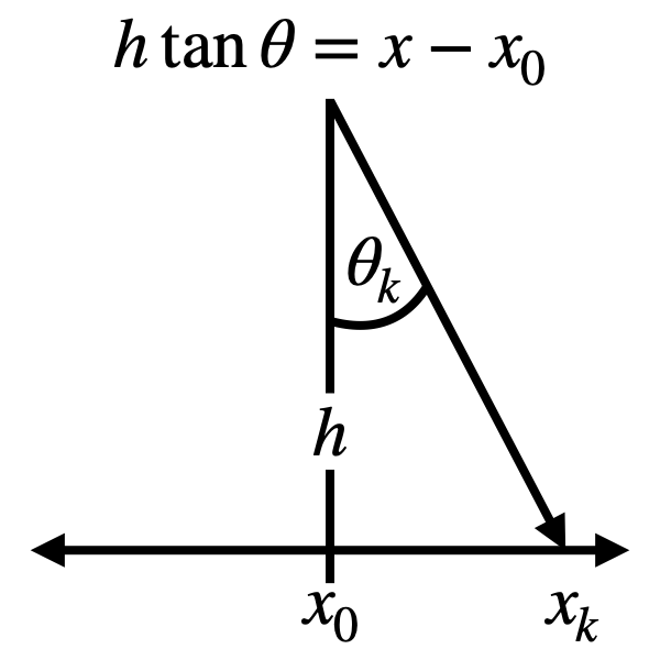
Relationship between \(\theta\) and \(x\). Here we want to consider the case where we don’t know anything about the underlying probability distribution of \(\theta\) other than that it is supported on \([-\pi/2, \pi/2]\) and that is is normalized, and we want this result as a distribution on \(x\). \(h\) and \(x_0\) are arbitrary parameters.

Since we have the relationship between \(\theta\) and \(x\), and the relationship is defined over \(\theta \in [-\pi/2,\pi/2]\), we can do a change of variables to get \(p(x)\) instead of \(p(\theta)\) and then carry out the maximization of entropy. To do the change of variables, we need

\[\begin{aligned} h \tan \theta &= x - x_0 \\ h \sec^2 \theta~d \theta &= dx \\ h (\tan^2 \theta + 1)~d \theta &= dx \\ h \left[\left(\frac{x - x_0}{h}\right)^2 + 1\right]~d \theta &= dx \\ \frac{1}{h}\left[\left(x - x_0\right)^2 + h^2 \right]~d\theta &= dx \\ d\theta &= \frac{h}{\left(\left(x - x_0\right)^2 + h^2 \right)} dx\end{aligned}\]

so that

\[p(\theta) = p(x) \left| \frac{dx}{d\theta}\right| = p(x) \frac{1}{h}\left[\left(x - x_0\right)^2 + h^2 \right]\]

For the limits on integration, we can easily see that

\(\tan (\pi/2) \to \infty\) and \(\tan (-\pi/2) \to -\infty\)

so \(x \in (-\infty,\infty)\). All together, we now want to maximize

\[\begin{aligned} H(p(\theta)) &= - \int_{-\pi/2}^{\pi/2} p(\theta)\ln p(\theta) d\theta \\ H(p(x)) &= - \int_{-\infty}^{\infty} \frac{p(x) \left(\left(x - x_0\right)^2 + h^2 \right)}{h}\ln \left[ \frac{p(x)\left(\left(x - x_0\right)^2 + h^2 \right)}{h}\right] \frac{h}{\left(\left(x - x_0\right)^2 + h^2 \right)} dx \\ &= - \int_{-\infty}^{\infty} p(x) \ln \left[ \frac{p(x)\left(\left(x - x_0\right)^2 + h^2 \right)}{h}\right]dx \\ &= - \int_{-\infty}^{\infty} p(x) \ln p(x) dx - \int_{-\infty}^{\infty} p(x) \ln \left[\frac{\left(\left(x - x_0\right)^2 + h^2 \right)}{h}\right]dx \end{aligned}\]

subject to \(\int_{-\infty}^{\infty} p(x) dx = 1\) therefore, our Lagrangian is

\[\begin{aligned} J(p(x),\lambda_0) &= - \int_{-\infty}^{\infty} p(x) \ln p(x) dx \\ &\quad - \int_{-\infty}^{\infty} p(x) \ln \left[\frac{\left(\left(x - x_0\right)^2 + h^2 \right)}{h}\right]dx \\ &\quad + \lambda_0 \left(\int_{-\infty}^{\infty} p(x) dx - 1\right) \end{aligned}\]

and carrying out the maximization yields

\[\frac{\partial J(p(x),\lambda_0)}{\partial p(x)} = -1 - \ln p(x) - \ln \left[\frac{\left(\left(x - x_0\right)^2 + h^2 \right)}{h}\right] + \lambda_0 = 0\]

which gives

\[\begin{aligned} p(x) &= \exp \left(\lambda_0 - 1 - \ln \left[\frac{\left(\left(x - x_0\right)^2 + h^2 \right)}{h}\right] \right) \\ &= \frac{h}{\left(\left(x - x_0\right)^2 + h^2 \right)} \exp (\lambda_0 - 1) \end{aligned}\]

substituting this into the normalization condition allows us to eliminate the \(\lambda_0\)

\[\begin{aligned} \int_{-\infty}^{\infty} \frac{h}{\left(\left(x - x_0\right)^2 + h^2 \right)} \exp (\lambda_0 - 1)dx &= 1 \\ \exp (\lambda_0 - 1) \int_{-\infty}^{\infty} \frac{h}{\left(\left(x - x_0\right)^2 + h^2 \right)}dx &= 1 \\ \exp (\lambda_0 - 1) \pi &= 1 \\ \exp (\lambda_0 - 1) &= 1/\pi \end{aligned}\]

therefore, we get

\[p(x) = \frac{h}{\pi\left(\left(x - x_0\right)^2 + h^2 \right)}\]

So for sampling random angles and not knowing anything about the underlying distribution (e.g. \(\theta\) is continuous uniform), we see that the resulting distribution over \(x\) is a Cauchy distribution, when \(x\) and \(\theta\) have the relationship illustrated above.

Exponential distribution

Now extend the continuous distribution to the case where we have a known expected value of \(x = \mu\). We will limit ourselves to the support \([0,\infty)\). As before we maximize

\[H(p(x)) = - \int_0^\infty p(x)\ln p(x) dx\]

but now subject to

\[\int_0^\infty p(x) dx = 1, \qquad \int_0^\infty x p(x) dx = \mu\]

which gives us our Lagrangian

\[J(p(x),\lambda_0, \lambda_1) = - \int_0^\infty p(x)\ln p(x) dx + \lambda_0 \left(\int_0^\infty p(x) dx - 1\right) + \lambda_1 \left(\int_0^\infty x p(x) dx - \mu\right)\]

differentiating the above with respect to \(p(x)\) and setting to zero gives

\[\begin{aligned} \frac{\partial J(p(x),\lambda_0, \lambda_1)}{\partial p(x)} &= \frac{\partial}{\partial p(x)} \left(- \int_0^\infty p(x)\ln p(x) dx + \lambda_0 \left(\int_0^\infty p(x) dx - 1\right)+ \lambda_1 \left(\int_0^\infty x p(x) dx - \mu\right)\right) \\ &= -\ln p(x) - 1 + \lambda_0 +\lambda_1 x = 0. \end{aligned}\]

which gives us an expression for \(p(x)\) as

\[p(x) = \exp \left(\lambda_0 - 1\right) \exp(\lambda_1 x)\]

this results in the following expressions for our constraints:

\[\int_0^\infty p(x) dx = \exp \left(\lambda_0 - 1\right) \int_0^\infty \exp(\lambda_1 x) dx = \exp \left(\lambda_0 - 1\right) \left(\frac{-1}{\lambda_1}\right) = 1\]

where \(\frac{-1}{\lambda_1} < 0\) in order for the integral to converge. For the second constraint we have

\[\int_0^\infty x p(x) dx = \exp \left(\lambda_0 - 1\right) \int_0^\infty x \exp(\lambda_1 x) dx = \exp \left(\lambda_0 - 1\right) \left(\frac{1}{\lambda_1^2}\right) = \mu\]

Dividing the two constraints by each other allows us to solve for \(\lambda_1\):

\[\frac{\exp \left(\lambda_0 - 1\right)}{\exp \left(\lambda_0 - 1\right)}\frac{-1/\lambda_1}{1/\lambda_1^2} = -\lambda_1 = 1/\mu\]

and then from the normalization we get

\[\exp \left(\lambda_0 - 1\right) \int_0^\infty \exp(-x/\mu) dx = \exp \left(\lambda_0 - 1\right) \mu = 1\]

which means \(\exp \left(\lambda_0 - 1\right) = 1/\mu\) and so from knowing a fixed mean, we obtain the exponential distribution over \([0,\infty)\)

\[p(x) = \frac{1}{\mu} \exp \left(-\frac{x}{\mu}\right)\]

Gaussian distribution

Now consider the case where we have a known mean \(\mu\) and variance \(\sigma^2\). We will consider \(x \in (-\infty,\infty)\). Because variance is the expectation of the squared deviation of a random variable \(x\) from its mean, it suffices to introduce the constraint

\[\int_{-\infty}^\infty (x - \mu)^2 p(x) dx = \sigma^2\]

which we will consider along with normalization when maximizing the entropy. This leads to the Lagrangian

\[J(p(x),\lambda_0, \lambda_1) = - \int_{-\infty}^\infty p(x)\ln p(x) dx + \lambda_0 \left(\int_{-\infty}^\infty p(x) dx - 1\right) + \lambda_1 \left(\int_{-\infty}^\infty (x- \mu)^2 p(x) dx - \sigma^2\right)\]

which, when differentiated with respect to \(p(x)\) and set equal to zero, yields

\[\frac{\partial J(p(x),\lambda_0, \lambda_1)}{\partial p(x)} = -\ln p(x) - 1 + \lambda_0 +\lambda_1 (x - \mu)^2 = 0\]

which gives us an expression for \(p(x)\) as

\[p(x) = \exp \left(\lambda_0 - 1\right) \exp(\lambda_1 (x-\mu)^2)\]

For the first constraint, we find that

\[\begin{aligned} \int_{-\infty}^\infty p(x) dx &= 1 \\ \int_{-\infty}^\infty \exp \left(\lambda_0 - 1\right) \exp(\lambda_1 (x-\mu)^2) dx &= 1 \\ \exp \left(\lambda_0 - 1\right) \int_{-\infty}^\infty \exp(\lambda_1 (x-\mu)^2) dx &= 1 \\ \exp \left(\lambda_0 - 1\right) \sqrt{\frac{\pi}{-\lambda_1}} &= 1 \\ \exp \left(\lambda_0 - 1\right) &= \sqrt{\frac{-\lambda_1}{\pi}} . \end{aligned}\]

And for the second constraint we find

\[\begin{aligned} \int_{-\infty}^\infty (x - \mu)^2 p(x) dx &= \sigma^2 \\ \int_{-\infty}^\infty \sqrt{\frac{-\lambda_1}{\pi}} (x - \mu)^2 \exp(\lambda_1 (x-\mu)^2) dx &= \sigma^2 \\ \sqrt{\frac{-\lambda_1}{\pi}} \int_{-\infty}^\infty (x - \mu)^2 \exp(\lambda_1 (x-\mu)^2) dx &= \sigma^2 \\ \sqrt{\frac{-\lambda_1}{\pi}} \cdot \frac{1}{2}\sqrt{\frac{\pi}{-\lambda_1^3}} &= \sigma^2 \\ \lambda_1 &= -\frac{1}{2\sigma^2}. \end{aligned}\]

Which allows us to say that

\[\exp \left(\lambda_0 - 1\right) = \frac{1}{\sqrt{2\pi\sigma^2}}\]

Putting this all together yields the Gaussian, or normal distribution

\[p(x) = \frac{1}{\sqrt{2\pi\sigma^2}}\exp\left(-\frac{(x-\mu)^2}{2\sigma^2}\right)\]

Bernoulli distribution

Moving back to the discrete case, let’s consider when a random variable \(k\) is either \(0\) or \(1\), i.e. \(k \in \{0,1\}\) and the expected value of \(k\) is \(\bar{p}\). This results in the Lagrangian

\[J(p_k, \lambda_0, \lambda_1) = -\sum_k p_k \ln p_k + \lambda_0\left(\sum_k p_k - 1\right) + \lambda_1 \left(\sum_k k p_k - \bar{p}\right)\]

Maximizing this Lagrangian gives

\[\frac{\partial J(p_k,\lambda_0)}{\partial p_k} = -1 - \ln p_k + \lambda_0 + \lambda_1 k = 0\]

which yields the probability mass function \(p_k\)

\[p_k = \exp \left(\lambda_0 - 1\right) \exp \left(\lambda_1 k \right)\]

Taking care of the first constraint,

\[\begin{aligned} \sum_k \exp \left(\lambda_0 - 1\right) \exp \left(\lambda_1 k \right) &= 1 \\ \exp \left(\lambda_0 - 1\right) \sum_k \exp \left(\lambda_1 k \right) &= 1 \\ \exp \left(\lambda_0 - 1\right) &= \frac{1}{\sum_k \exp \left(\lambda_1 k \right)} \\ \exp \left(\lambda_0 - 1\right) &= \frac{1}{\exp \left(\lambda_1 \cdot 0 \right) + \exp \left(\lambda_1 \cdot 1 \right)} \\ \exp \left(\lambda_0 - 1\right) &= \frac{1}{1 + \exp \left(\lambda_1 \right)} \end{aligned}\]

since \(k\) is either \(0\) or \(1\). Taking care of the second constraint,

\[\begin{aligned} \sum_k k \cdot \exp \left(\lambda_0 - 1\right) \exp \left(\lambda_1 k \right) &= \bar{p} \\ \exp \left(\lambda_0 - 1\right) \sum_k k \cdot \exp \left(\lambda_1 k \right) &= \bar{p} \\ \frac{\exp \left(\lambda_1 \right)}{1 + \exp \left(\lambda_1 \right)} &= \bar{p} \end{aligned}\]

again, since \(k\) is either \(0\) or \(1\). Then we can solve for \(\lambda_1\),

\[\lambda_1 = \ln \left( \frac{\bar{p}}{1-\bar{p}} \right)\]

which means that

\[\exp \left(\lambda_0 - 1\right) = \frac{1}{1 + \frac{\bar{p}}{1-\bar{p}}} = (1-\bar{p})\]

Putting this all together we have

\[\begin{aligned} p_k &= (1 - \bar{p}) \exp \left( k \cdot \ln \left(\frac{\bar{p}}{1-\bar{p}}\right)\right) \\ &= (1 - \bar{p}) \left(\frac{\bar{p}}{1-\bar{p}}\right)^k \\ &= \bar{p}^k (1 - \bar{p})^{k-1} \end{aligned}\]

Which is the Bernoulli distribution

\[p_k = \bar{p}^k (1 - \bar{p})^{k-1}\]

for when \(0 \leq \bar{p} \leq 1\) and \(k\) is either \(0\) or \(1\).

Binomial distribution

This is the case where we compute the probability for having \(N\) successes in \(M\) trials. The constraint here is the expected number of successes \(\langle N \rangle\). Note that this will depend on the number of trials, and since we only care abut the number of successes, and not the order in which they were taken, we need to use the generalized form of entropy

\[H(p) = -\sum_N^M p_N \ln \frac{p_N}{m(N)}\]

where \(m(N)\) is the Lebesgue measure, which accounts for the fact that we need to account for the fact that we are indifferent to the number of ways \(N\) can be accomplished. This is essentially the prior probability we assign to the different outcomes. For example, in the uniform distribution we had no reason to favor one proposition \(p_i\) over another, thus the principle of indifference led us to assign \(m(i) = 1\) for all \(i\), and the result led to each outcome being equally likely. But this is not always the case in combinatoric problems, for example, since (without replacement) there are 4 ways to pick a unique object out of a set of 4 unique objects, but 6 ways to pick out 2 objects out of the same set. So we would not expect the probabilities for 2 objects to be on the same scale as picking out 1 object; our prior information leads us to favor 4 choose 2 over 4 choose 1 – there are more ways it could happen. The measure \(m(N)\) allows us to account for that.

In other words, for this combinatoric problem,

\[m(N) = M!/N!(M-N)!\]

(As a chemist, I think of \(m(N)\) as event degeneracy.) Now, moving on, we are in addition to the normal entropy and normalization, constrained by the information \(\sum_N^M N p_N = \langle N \rangle = \mu\) Therefore, our Lagrangian reads

\[J(p_N,\ldots) = -\sum_N^M p_N \ln \frac{p_N}{m(N)} + \lambda_0 \left(\sum_N^M p_N - 1\right) + \lambda_1 \left(\sum_N^M N p_N - \mu\right)\]

which leads to the maximization

\[\frac{\partial J}{\partial p_N} = 0 = -1 - \ln \frac{p_N}{m(N)} + \lambda_0 + \lambda_1 N\]

so that

\[\begin{aligned} p_N &= m(N) \cdot \exp \left(\lambda_0 -1\right) \exp\left( \lambda_1 \right)^N \\ &= \frac{M!}{N!(M-N)!} \exp \left(\lambda_0 -1\right) \exp\left( \lambda_1 \right)^N \end{aligned}\]

and we chose the combinatoric measure because for each possible number of successes \(N\), there are \(M!/N!(M-N)!\) different ways of achieving this given \(M\) trials.

Solving for the first constraint:

\[\begin{aligned} 1 &= \sum_N^M p_N = \exp \left(\lambda_0 -1\right) \sum_N^M \frac{M!}{N!(M-N)!} \exp\left( \lambda_1 \right)^N \cdot (1)^{M-N} \\ &= \exp \left(\lambda_0 -1\right) \exp\left( \lambda_1 + 1\right)^M \\ &\implies \exp \left(\lambda_0 -1\right) = \exp\left( \lambda_1 + 1\right)^{-M} \end{aligned}\]

where we multiplied by \(1\) to the power of \(M-N\), which just equals one, in the first line in order to make use of the binomial formula and eliminate the sum. The inversion in the last line is made possible because the exponential is always greater than zero.

For the next constraint,

\[\begin{aligned} \mu &= \sum_N^M N \exp\left( \lambda_1 + 1\right)^{-M} \frac{M!}{N!(M-N)!} \exp\left( \lambda_1 \right)^N \\ &= \exp\left( \lambda_1 + 1\right)^{-M} \sum_N^M N \frac{M!}{N!(M-N)!} \exp\left( \lambda_1 \right)^N \\ &= \exp\left( \lambda_1 + 1\right)^{-M} \cdot \exp \left(\lambda_1\right) \cdot M \cdot \left( \exp\left( \lambda_1 \right) + 1 \right)^{M-1} \\ &= M \cdot \frac{\exp(\lambda_1)}{\exp(\lambda_1) + 1} \end{aligned}\]

In fairness, I used WolframAlpha to finally eliminate the sum after the second line. If we let \(p \leftarrow \mu/M\), then we can finally see that

\[\begin{aligned} \exp(\lambda_1) = \frac{p}{1-p}\end{aligned}\]

which we can obtain because \(p > 0\).

Okay. Putting it all together now:

\[\exp \left(\lambda_0 -1\right) = \left(\frac{p}{1-p} + 1 \right)^{-M} = \left(\frac{1}{1-p}\right)^{-M} = \left( 1-p \right)^M\]

and

\[\exp \left(\lambda_1 \right)^N = \left(\frac{p}{1-p}\right)^{N} = \left(\frac{1-p}{p}\right)^{-N} = \left(\frac{1}{p} - 1 \right)^{-N}\]

which lets us finally show that

\[p_N = \frac{M!}{N!(M-N)!} \cdot \left( 1-p \right)^M \cdot \left(\frac{1}{p} - 1 \right)^{-N}\]

or, simply,

\[p_N = \frac{M!}{N!(M-N)!} \left(p \right)^{N} \left( 1-p \right)^{M-N}\]

which is the binomial distribution.

Others

There are plenty others, like the Poisson, beta, and von Mises distributions which can be derived in a like manner. I may add more here if I get to it. Until then, check out the table from Wikipedia.