I had my second first author paper published a few weeks back in the Journal of Physical Chemistry A, and wanted to share it here. It’s an investigation of how the tiny little hydrogen molecule binds to open metal sites in metal organic frameworks.
Metal organic frameworks are like molecular sponges. They are very porous and small gases seem drawn to them, so researchers want to use them to store hydrogen gas for fuel cells. Another interesting use is to use them for purifying gases! Imagine if we could store and condense carbon dioxide right out of the air! Lots of potential environmental applications — problem is, no one really knows how they work.
We studied the hydrogen gas binding to a series of different metals in these metal organic frameworks. Here is a picture of one of the systems we studied. 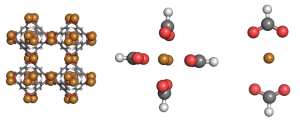 The full metal organic framework is on the left. To simplify our method, we made ‘mimics’, meaning we studied just one part of a metal organic framework. That’s what you see in the center and on the right. Here is a close up of an interaction
 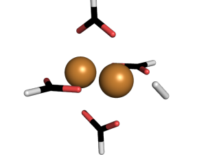 Hydrogen is kind of weird in that it has no charge and only two electrons. So why does bind to the metal centers? To understand why, we used a method called Symmetry Adapted Perturbation Theory (SAPT). This method was designed to study weak interactions between molecules. In addition to calculating the energy of the hydrogen sticking to the metal, it also decomposes the interaction into physical forces: like electrostatic, dispersion, induction, etc. It can be an extremely accurate method (we compared it to CCSD(T) energies and got pretty much the same results).
What we found might surprise you, as it did me! Hydrogen binds weakly (like ~ 3 kcal/mol weakly) and in many cases a good third of the interaction comes from dispersion forces. Now, if you remember from general chemistry, the more electrons you have, the greater the effects of dispersion become. Yet hydrogen — that little H2, with only two electrons — had an interaction largely mediated by dispersion (electrostatics was the other major component, which wasn’t too surprising).
The conclusion? Don’t ignore (or underestimate) your dispersion forces! This is very important to researchers who continue to study these metal organic frameworks, as they like to use density functional theory (DFT), which has some problems describing dispersion (if you aren’t careful).
You can read the whole paper here.
Kinetic balance was discovered when early attempts at relativistic SCF calculations failed to converge to a bound state. Often, the energy was too low because of the negative energy continuum. The crux of the problem was that the four components of the spinor in relativistic methods were each allowed to vary independently. In other words, scientists treated each component with its own, independent basis without regard to how the components depended on each other. This problem was eventually solved by paying attention to the non-relativistic limit of the kinetic energy, and noting that the small and large components of the four-spinor are not independent. There is, in fact, a coupling that we refer to as ‘‘kinetic balance’’. I’ll show you how it works.
First, as you may have guessed, we only need to consider the one-electron operator. This is the matrix form of the Dirac equation, and it contains (in addition to other terms) the contributions to the kinetic energy. Written as a pair of coupled equations, we have
\[\begin{array}{c} \left[\mathbf{V}^{LL} - E \mathbf{S}^{LL} \right] \mathbf{c}^L + c \mathbf{\Pi}^{LS} \mathbf{c}^S = 0 \\ c \mathbf{\Pi}^{SL} \mathbf{c}^L + \left[\mathbf{V}^{SS} - (2mc^2 + E)\mathbf{S}^{SS}\right]\mathbf{c}^S = 0 \end{array} \ \ \ \ \ (1)\]
Where \({\mathbf{V}^{LL} = \langle \chi^{L} \vert V \vert \chi^{L} \rangle}\), \({\mathbf{S}^{LL} = \langle \chi^{L} \vert \chi^{L} \rangle}\), and \({\mathbf{\Pi}^{LS} = \langle \chi^{L} \vert -i\hbar \mathbf{\sigma} \cdot \mathbf{\nabla} \vert \chi^{S} \rangle}\), and so on. These are the potential, overlap, and momentum terms of the Dirac equation in a basis \({\vert \chi \rangle}\).
Now, if we look at the second of the two paired equations, we note that for potentials of chemical interest (e.g. molecular or atomic), \({\mathbf{V}^{SS}}\) is negative definite. We also know that when we solve the equation, we are looking for and energy above the negative energy continuum, which is to say we want \({E \> -2mc^2}\). Since the overlap is positive definite, putting all of these constraints together mean that we have a nonsingular matrix (and therefore invertible!) matrix in the second of our coupled equations. We can rewrite the second equation as
\[\mathbf{c}^S = \left[(2mc^2 + E)\mathbf{S}^{SS} - \mathbf{V}^{SS} \right]^{-1}c\mathbf{\Pi}^{SL} \mathbf{c}^L \ \ \ \ \ (2)\]
Substituting this expression back into the first (top) equation yields
\[\left[\mathbf{V}^{LL} - E \mathbf{S}^{LL} \right] \mathbf{c}^L + c \mathbf{\Pi}^{LS} \left[(2mc^2 + E)\mathbf{S}^{SS} - \mathbf{V}^{SS} \right]^{-1}c\mathbf{\Pi}^{SL} \mathbf{c}^L = 0 \ \ \ \ \ (3)\]
This form is very useful for analysis. Now, we are going to use the matrix relation
\[(\mathbf{A} - \mathbf{B})^{-1} = \mathbf{A}^{-1} + \mathbf{A}^{-1}\mathbf{B}(\mathbf{A}-\mathbf{B})^{-1} \ \ \ \ \ (4)\]
with \({\mathbf{A} = 2mc^2\mathbf{S}^{SS}}\) and \({\mathbf{B} = \mathbf{V}^{SS} - E\mathbf{S}^{SS}}\). This leads to the rather long expression
\[\begin{array}{c} \left[\mathbf{V}^{LL} - E\mathbf{S}^{LL} + \frac{1}{2m} \mathbf{\Pi}^{LS} \left[\mathbf{S}^{SS}\right]^{-1}\mathbf{\Pi}^{SL}\right] \mathbf{c}^{L} = \cdots \\ \cdots = \frac{1}{2m}\mathbf{\Pi}^{LS}\left[\mathbf{S}^{SS}\right]^{-1} \left[\mathbf{V}^{SS} - E\mathbf{S}^{SS}\right]\left[\mathbf{V}^{SS} - (2mc^2+E)\mathbf{S}^{SS}\right]^{-1} \mathbf{\Pi}^{SL}\mathbf{c}^{L} \end{array} \ \ \ \ \ (5)\]
Why this ridiculous form? Look closely at each side and their dependence on the speed of light, \({c}\). The left hand side has the \({c^0}\) terms, and the right hand side has the \({c^{-2}}\) terms. Since the non relativistic limit is found when the speed of light is infinite (\({c \rightarrow \infty}\)), the whole right hand side goes to zero. This gives us
\[\left[\mathbf{V}^{LL} - E\mathbf{S}^{LL} + \frac{1}{2m} \mathbf{\Pi}^{LS} \left[\mathbf{S}^{SS}\right]^{-1}\mathbf{\Pi}^{SL}\right] \mathbf{c}^{L} = 0 \ \ \ \ \ (6)\]
Now, if this is indeed the true non-relativistic limit, then we find that our kinetic energy term \({\mathbf{T}^{LL}}\) is given by
\[\mathbf{T}^{LL} = \frac{1}{2m} \mathbf{\Pi}^{LS} \left[\mathbf{S}^{SS}\right]^{-1}\mathbf{\Pi}^{SL} \ \ \ \ \ (7)\]
Or, more explicitly,
\[T^{LL}_{\mu \nu} = \frac{-\hbar^2}{2m} \sum\limits_{\kappa \lambda} \langle \chi_{\mu}^{L} \vert \mathbf{\sigma}\cdot\mathbf{\nabla}\vert \chi_{\kappa}^{S} \langle \left[S^{SS}\right]_{\kappa \lambda}^{-1} \langle \chi_{\lambda}^{S} \vert \mathbf{\sigma} \cdot \mathbf{\nabla} \vert \chi_{\nu}^{L} \rangle \ \ \ \ \ (8)\]
Where that inner part, \({\vert \chi_{\kappa}^{S} \langle \left[S^{SS}\right]_{\kappa \lambda}^{-1} \langle \chi_{\lambda}^{S} \vert }\), is an inner projection onto the small component basis space. Less formally, the small component is the ‘‘mathematical glue’’ that connects the two momentum operators. If the small component spans the same space as the momentum operators in the large component space, \({\{\sigma\cdot\nabla\chi_{\mu}^{L}\}}\), then that inner projection just becomes the identity. This means that the expression becomes
\[T_{\mu \nu} = \frac{-\hbar^2}{2m}\langle \chi_{\mu}^{L} \vert (\mathbf{\sigma}\cdot\mathbf{\nabla})(\mathbf{\sigma} \cdot \mathbf{\nabla}) \vert \chi_{\nu}^{L} \rangle = \frac{-\hbar^2}{2m} \langle \chi_{\mu}^{L} \vert \mathbf{\nabla}^2 \vert \chi_{\nu}^{L} \rangle \ \ \ \ \ (9)\]
Which is the kinetic energy term in the non-relativistic formulation! (N.B. We used the relation \({(\mathbf{\sigma}\cdot\mathbf{\nabla})(\mathbf{\sigma}\cdot\mathbf{\nabla}) = \mathbf{\nabla}^2}\)).
So, when we set up our relativistic calculations, as long as we have the constraint that
\[\chi_{\mu}^{S} = (\mathbf{\sigma}\cdot\mathbf{p})\chi_{\mu}^{L} \ \ \ \ \ (10)\]
Then we will find that we recover the correct non-relativistic limit of our equations. The basis is called ‘‘kinetically balanced’’, and we won’t collapse to energies lower than \({-2mc^2}\).
A few stray observations before we finish. First, if we enforce the relation between small and large component basis functions, then we find that \({\mathbf{\Pi}^{SL} = \mathbf{S}^{SS}}\) and \({\mathbf{\Pi}^{LS} = 2m\mathbf{T}^{LL} = 2m\mathbf{T}}\). Second, this constraint actually maximizes kinetic energy, and any approximation that does not satisfy the kinetic balance condition will lower the energy. This was weird to me coming from the non relativistic Hartree-Fock background, where variationally, if you remove basis functions you raise the energy. The thing is that when doing relativistic calculations, you aren’t bounded from below like their non-relativistic counterparts. While you can get variational stability, you are actually doing an ‘‘excited state’’ calculation (I am using the term ‘‘excited state’’ very loosely). Kind of odd, but the negative energy continuum does exist, and was a big factor in the predicting the existence of antimatter.
Finally, modern methods of relativistic electronic structure theory make use of the kinetic balance between large and small component basis functions to eliminate the small component completely. These are called ‘‘Dirac-exact’’ methods. One such example is NESC, or Normalized Elimination of the Small Component. In addition to reproducing the Dirac equation exactly, they have numerous computational benefits, as well as easily allowing for most (if not all) non-relativistic correlated methods to be applied directly. Thus after doing an NESC calculation, you get relativistic ‘‘orbitals’’ which can immediately be used in, say, a coupled cluster calculation with no computational modification.
Comments, questions, or corrections? Let me know!
I wanted to try and understand more of how the physical picture changes going from non-relativistic theories to relativistic theories in electronic structure theory. So I figured a good place to start would be with the relativistic analog to the Hartree-Fock theory we know and love so well :)
Why do I care about relativistic electronic structure theory? It is the most fundamental theory of molecular science we have available! In particular, it is the most natural way to model and understand spin in molecules: molecular magnets, spin-orbit couplings, and high-energy spectroscopy all intrinsically depend on a theory of molecules that includes special relativity and a first principles treatment of spin. It also explains the reactivity (or lack thereof) of heavy metals, as well as their colors and properties. Did you know that if we did not include special relativity in our theories we’d predict gold to be silver instead of yellow? It’s just one of the reasons I think the next decade or so will refine relativistic electronic structure theory into the de facto theory of molecules. Kind of like what coupled cluster did to the electron correlation problem over the past few decades, relativistic theories are maturing fast and should become standard in your favorite quantum chemistry packages. Anyway…
The Dirac-Hartree-Fock (DHF) operator for a single determinant wave function in terms of atomic spinors is identical to that in terms of atomic orbitals. The derivation is the same: you find the energetic stationary point with respect to spinor (orbital) rotations. Thus we start with the DHF operator:
\[f_{pq} = h_{pq} + \sum\limits_{i}^{N} \left( pq \vert \vert ii \right) \ \ \ \ \ (1)\]
The first term, \({h_{pq}}\), is the one-electron part. The second term is the two-electron part. We will look at the one-electron part first. For \({h_{pq}}\), we (obviously) cannot use the Schrödinger equation equivalent. Instead, we use the Dirac equation, which is the relativistic equation for a single electron. In two-spinor form, where
\[\psi = \left( \begin{array}{c} \psi^{L} \\ \psi^{S} \end{array} \right) \ \ \ \ \ (2)\]
(Which is to say \({\psi^{L}}\) is the large component and \({\psi^{S}}\) is the small component.) We have the expression
\[\left[\begin{array}{cc} V-E & c(\mathbf{\sigma}\cdot\mathbf{p}) \\ c(\mathbf{\sigma}\cdot\mathbf{p}) & V-E-2mc^2 \end{array} \right] \left[\begin{array}{c} \psi^{L} \\ \psi^{S} \end{array} \right] = 0 \ \ \ \ \ (3)\]
In this case \({c}\) is the speed of light and \({m}\) is the electron rest mass. \({V}\) is the potential, which in the non-relativistic case is the point charge nucleus, though in general relativistic quantum chemistry assumes a finite nucleus. The bold operators are vectors, for example momentum \({\mathbf{p} = (p_x, p_y, p_z)}\). Same with the Pauli operators. Now we will expand \({\psi^L}\) and \({\psi^S}\) in a basis. Again, the bold type means a vector.
\[\psi^L = \vert \chi^L \rangle \mathbf{c}^L; \qquad \psi^S = \vert \chi^S \rangle \mathbf{c}^S \ \ \ \ \ (4)\]
The \({\mathbf{c}}\) is a column vector containing the basis coefficients, just like in non-relativistic Hartree-Fock theory. Similarly, the \({\vert \chi \rangle}\) ket is our basis. Inserting these expressions and multiplying on the left by \({\left[\langle \chi^L \vert \quad \langle \chi^S \vert \right]}\) (compare with Szabo and Ostlund p. 137) we transform the integro-differential equations into a matrix equation.
\[\left[\begin{array}{cc} \langle \chi^L \vert V \vert \chi^L \rangle - E\langle \chi^L \vert \chi^L \rangle & c\langle \chi^L \vert -i\hbar \mathbf{\sigma}\cdot\mathbf{\nabla} \vert \chi^S \rangle \\ c\langle \chi^S \vert -i\hbar \mathbf{\sigma}\cdot\mathbf{\nabla} \vert \chi^L \rangle & \langle \chi^S \vert V \vert \chi^S \rangle - (2mc^2 +E) \langle \chi^S \vert \chi^S \rangle \end{array} \right] \left[\begin{array}{c} \mathbf{c}^L \\ \mathbf{c}^S \end{array} \right] = 0 \ \ \ \ \ (5)\]
Which, we will simplify to
\[\left[\begin{array}{cc} \mathbf{V}^{LL} - E\mathbf{S}^{LL} & c\mathbf{\Pi}^{LS} \\ c\mathbf{\Pi}^{SL} & \mathbf{V}^{SS} - (2mc^2 +E) \mathbf{S}^{SS} \end{array} \right] \left[\begin{array}{c} \mathbf{c}^L \\ \mathbf{c}^S \end{array} \right] = 0 \ \ \ \ \ (6)\]
Hopefully, it is obvious we made the notational replacements
\[\mathbf{V}^{LL} = \langle \chi^L \vert V \vert \chi^L \rangle; \quad \mathbf{S}^{LL} = \langle \chi^L \vert \chi^L \rangle; \quad \mathbf{\Pi}^{LS} = \langle \chi^L \vert -i\hbar \mathbf{\sigma}\cdot\mathbf{\nabla} \vert \chi^S \rangle; ~\hbox{etc.} \ \ \ \ \ (7)\]
For the DHF equations, we will slide the parts containing energy \({E}\) over to the right hand side to recover the eigenvalue equation. We must now consider the analog to the Coulomb and exchange integrals in the non-relativistic HF equations to the relativistic Dirac equations. There are a few extra things to consider. The first is made clearest if we recall the definition of the two electron integrals (in Mulliken notation) for the non relativistic case. In general, we have
\[(pq\vert rs) = \int\int \psi^{*}_p(\mathbf{r}_1) \psi_q(\mathbf{r}_1) \frac{1}{r_{12}} \psi^{*}_r(\mathbf{r}_2) \psi_s(\mathbf{r}_2)d\mathbf{r}_1d\mathbf{r}_2 \ \ \ \ \ (8)\]
In the relativistic case, we swap the orbitals \({\psi}\) with their four-component spinors. We will have the same equation as above, except instead of the complex conjugate, we have the adjoint.
\[(pq\vert rs) = \int\int \psi^{\dagger}_p(\mathbf{r}_1) \psi_q(\mathbf{r}_1) \frac{1}{r_{12}} \psi^{\dagger}_r(\mathbf{r}_2) \psi_s(\mathbf{r}_2)d\mathbf{r}_1d\mathbf{r}_2 \ \ \ \ \ (9)\]
This slight change is just because we aren’t dealing with scalar functions anymore. For the most part things stay the same (at least in appearance), and we deal with charge distributions between two four spinors (in two spinor form) like so:
\[\psi_p^{\dagger}\psi_q = \left( \psi_p^{L\dagger} \psi_p^{S\dagger} \right) \left( \begin{array}{c} \psi_q^{L} \\ \psi_q^S \end{array} \right) = \psi_p^{L\dagger}\psi_q^{L} + \psi_p^{S\dagger}\psi_q^{S} \ \ \ \ \ (10)\]
So it is ever so slightly more involved, but nothing too out of the ordinary. Extending this idea to the two electron integrals gives
\[(pq\vert rs) = (p^{L}q^{L}\vert r^{L}s^{L}) + (p^{L}q^{L}\vert r^{S}s^{S}) + (p^{S}q^{S}\vert r^{L}s^{L}) + (p^{S}q^{S}\vert r^{S}s^{S}) \ \ \ \ \ (11)\]
Okay. Now implicit to all of this so far is that the interaction between two charge densities is just Coulombic and hasn’t changed going from non relativistic to relativistic theories. This is not really the case, because the Coulombic interaction assumes an instantaneous response between electrons. QED tells us that this interaction is mediated by photons and therefore the interaction cannot occur any faster than the speed of light. In other words, there is a retardation effect between electrons that we must account for. This correction to the Coulomb interaction is called the Breit interaction, given by
\[V^{C}(0,r_{ij}) = \frac{1}{r_{ij}} - \frac{\mathbf{\alpha_i}\cdot\mathbf{\alpha}_j}{r_{ij}} + \frac{(\mathbf{\alpha}_i \times r_{ij})(\mathbf{\alpha}_j \times r_{ij})}{r_{ij}^3} \ \ \ \ \ (12)\]
We will ignore this for the rest of the derivation (thus ultimately giving the Dirac-Coulomb-Hartree-Fock equations), but to see how the interaction may be accounted for, consider that you now have new integrals that take the form
\[\psi_p^{\dagger}\mathbf{\alpha}\psi_q = \left( \psi_p^{L\dagger} \psi_p^{S\dagger} \right) \left( \begin{array}{cc} 0_2 & \mathbf{\sigma} \\ \mathbf{\sigma} & 0_2 \end{array} \right) \left( \begin{array}{c} \psi_q^{L} \\ \psi_q^S \end{array} \right) = \psi_p^{S\dagger}\mathbf{\sigma}\psi_q^{L} + \psi_p^{L\dagger}\mathbf{\sigma}\psi_q^{S} \ \ \ \ \ (13)\]
Which basically adds some different coupling elements. The alpha is the dame as in the Dirac equation, and the sigma is again your Pauli matrices. Anyway, going back, we now have a form of the two-electron integrals in 2-spinor form. We can insert the same basis set expansion elements as before for the one-electron case, and we get, for example
\[(p^L q^L \vert r^L s^L) = \sum\limits_{\mu \nu \kappa \lambda} c^{L*}_{\mu p} c^{L}_{\nu q} c^{L*}_{\kappa r} c^{L}_{\lambda s} (\mu^L \nu^L \vert \kappa^L \lambda^L) \ \ \ \ \ (14)\]
And similar expressions hold for the other terms. This should look nearly identical to the molecular-orbital/atomic-orbital relation in Hartree Fock theory.
And that’s really all there is to it! To clean up our expressions, we introduce density matrix \({\mathbf{P}}\), where, for example
\[\mathbf{P} = \left[\begin{array} {cc} \mathbf{P}^{LL} & \mathbf{P}^{LS} \\ \mathbf{P}^{SL} & \mathbf{P}^{SS} \end{array} \right] \ \ \ \ \ (15)\]
with
\[\mathbf{P}^{LL} = \mathbf{c}^{L}\mathbf{c}^{L\dagger}, ~\hbox{etc.} \ \ \ \ \ (16)\]
Then our Dirac-(Coulomb-) Hartree Fock matrix looks like
\[\mathbf{F} = \left[\begin{array} {cc} \mathbf{F}^{LL} & \mathbf{F}^{LS} \\ \mathbf{F}^{SL} & \mathbf{F}^{SS} \end{array} \right] \ \ \ \ \ (17)\]
With
\[F^{LL}_{\mu \nu} = V^{LL}_{\mu \nu} + \sum\limits_{\kappa \lambda} P^{LL}_{\kappa \lambda} \left[(\mu^L \nu^L \vert \kappa^L \lambda^{L}) - (\mu^{L} \lambda^{L} \vert \kappa^{L} \nu^{L})\right] + \sum\limits_{\kappa\lambda} P^{SS}_{\kappa \lambda} \left[(\mu^L \nu^L \vert \kappa^S \lambda^S )\right] \ \ \ \ \ (18)\]
\[F^{LS}_{\mu \nu} = c \Pi^{LS}_{\mu \nu} - \sum\limits_{\kappa \lambda} P_{\kappa \lambda}^{SL} (\mu^L \lambda^L \vert \kappa^{S} \nu^{S} ) \ \ \ \ \ (19)\]
\[F^{SS}_{\mu \nu} = V^{SS}_{\mu \nu} - 2c^2 S^{SS}_{\mu\nu} + \sum\limits_{\kappa \lambda} P_{\kappa \lambda}^{LL} (\mu^S \nu^S \vert \kappa^L \lambda^L) + \sum\limits_{\kappa \lambda} P_{\kappa \lambda}^{SS} \left[(\mu^S \nu^S \vert \kappa^S \lambda^S) - (\mu^S \lambda^S \vert \kappa^S \nu^S ) \right] \ \ \ \ \ (20)\]
And of course the form of the DHF equations is the same as in the non-relativistic case (with \({\mathbf{C}}\) the matrix of all eigenvectors \({\mathbf{c}}\)):
\[\mathbf{FC} = \mathbf{SC}E \ \ \ \ \ (21)\]
The Dirac Fock matrix is Hermitian, and you can see that it depends on the density \({\mathbf{P}=\mathbf{CC^{\dagger}}}\) as well, meaning we have to solve the equations iteratively.
Now, there is still a lot more to do with these equations, such as finding a suitable basis set and actually setting up the problem and integrals. It’s not a trivial task, but I plan to explore these more in the future.
Questions, comments, or corrections? Let me know! I’d love to hear from you.
According to Einstein’s special theory of relativity, the relation between energy (\({E}\)) and momentum (\({\mathbf{p}}\)) is given by the expression
\(E^2 = \mathbf{p}^2 c^2 + m_0^2 c^4 \ \ \ \ \ (1)\)
This relates a particle’s rest mass (\({m_0}\), which we will call \({m}\) from here on out), momentum, and total energy. This equation sets time and space coordinates on equal footing (a requirement for Lorentz invariance), and is a suitable starting point for developing a relativistic quantum mechanics. Now, when we derive non-relativistic quantum mechanics (the Schrödinger equation) we make use of the correspondence principle and replace classical momentum and energy with their quantum mechanical operators
\(E \rightarrow i\hbar \frac{\partial}{\partial t} \ \ \ \ \ (2)\)
and
\(\mathbf{p} \rightarrow -i \hbar \nabla \ \ \ \ \ (3)\)
It would make sense then, to extend this idea and substitute the operators into the relativistic energy-momentum expression. Doing so gives
\[\left(i\hbar \frac{\partial}{\partial t}\right)^2 = \left(-i\hbar \nabla \right)^2 c^2 + m^2 c^4 \ \ \ \ \ (4)\]
which reduces to (and is more commonly seen as)
\[\left( \frac{1}{c^2}\frac{\partial^2}{\partial t^2} - \nabla^2 + \frac{m^2 c^2}{\hbar^2} \right)\psi = 0 \ \ \ \ \ (5)\]
Where \({\psi}\) is our wave function. This equation is known as the Klein-Gordon equation and was one of the first attempts to merge special relativity with the Schrödinger equation. A couple things you might note about the Klein-Gordon equation right off the bat: first, it treats time and position equally as second order derivatives. This was one of the flaws in the non-relativistic Schrödinger equation, in that time was first order but position was second order. To be Lorentz invariant, and therefore a proper relativistic theory, both coordinates must be treated equally. The second thing you might notice is that the equation is spinless. Now, it turns out that the Klein-Gordon equation fails as a fundamental equation on account of not having a positive definite probability density. Probability can be negative in the Klein-Gordon equation! (Why? It turns out that having a time second derivative is the culprit. When integrating with respect to time, you can choose two independent integration constants for the wave function and its time derivative, which allow for both positive and negative probability densities.) Now, Feynman later re-interpreted the Klein-Gordon equation as an equation of motion for a spinless particle, so it isn’t completely useless. It also turns out that the Dirac equation (which is a fundamental equation) solutions will always be solutions for the Klein-Gordon equation, just not the other way around.
Okay, so the first attempt at deriving a relativistic Schrödinger equation didn’t quite work out. We still want to use the energy-momentum relation, and we still want to use the correspondence principle, so what do we try next? Since the second order time derivatives caused the problems for Klein-Gordon, so let’s try an equation of the form
\[E = \sqrt{\mathbf{p}^2 c^2 + m^2 c^4} = c\sqrt{\mathbf{p}^2 + m^2 c^2} \ \ \ \ \ (6)\]
If we then insert the corresponding operators, we get
\(i\hbar\frac{\partial}{\partial t} = c \sqrt{-\hbar^2 \nabla^2 + m^2c^2} \ \ \ \ \ (7)\)
Now as you might have guessed, this form presents some problems because we can’t easily solve for the square root of the squared momentum operator. We could try a series expansion of the form
\(i\hbar\frac{\partial}{\partial t} = mc^2 \sqrt{1 - \left(\frac{\hbar \nabla}{mc}\right)^2} = mc^2 - \frac{\hbar^2 \nabla^2}{2m} + \frac{\hbar^4 \nabla^4}{8m^3c^2} + \cdots \ \ \ \ \ (8)\)
But this gets quite complicated. Moreover, to be soluble we have to truncate at some point, and any truncation will destroy our Lorentz invariance. So we must look elsewhere to solve this problem. Dirac’s insight was to go back to the argument of the square root operator and assume that it could be written as a perfect square. In other words, determine \({\mathbf{\alpha}}\) and \({\beta}\) such that
\(\mathbf{p}^2 + m^2c^2 = \left(\mathbf{\alpha} \cdot \mathbf{p} + \beta m c\right)^2 \ \ \ \ \ (9)\)
If we do this, the square root goes away, and we get the Dirac equation for a free particle.
\(i\hbar\frac{\partial}{\partial t} \psi = c \alpha \cdot \left( - i \hbar \nabla \right) \psi + \beta mc^2 \psi \ \ \ \ \ (10)\)
Of course, we have said absolutely nothing about what \({\alpha}\) and \({\beta}\) actually are. We can see that \({\alpha}\) is going to have three components, just like momentum has \({x,y,z}\), and that \({\beta}\) will have a single component. To satisfy the perfect square’’ constraint, we can distill’’ out three constraints.
\(\alpha_i^2 = \beta^2 = 1, \qquad \alpha_i\alpha_j = - \alpha_j \alpha_i, i \neq j, \qquad \alpha_i\beta = -\beta\alpha_i \ \ \ \ \ (11)\)
Well, there is no way we are going to satisfy the constraints with \({\alpha}\) and \({\beta}\) as scalars! So let’s look to rank-2 matrices, such as the Pauli matrices:
\(\sigma_x = \begin{bmatrix} 0 & 1 \\ 1 & 0 \end{bmatrix} \ \ \ \ \ (12)\)
\[\sigma_y = \begin{bmatrix} 0 & -i \\ i & 0 \end{bmatrix} \ \ \ \ \ (13)\]
\[\sigma_z = \begin{bmatrix} 1 & 0 \\ 0 & -1 \end{bmatrix} \ \ \ \ \ (14)\]
and the identity
\(\mathbf{I}_2 = \begin{bmatrix} 1 & 0 \\ 0 & 1 \end{bmatrix} \ \ \ \ \ (15)\)
Well, while it might seem like these would work, unfortunately, we have to include the identity. Because the identity commutes with all of the rank-2 matrices, we will never get the proper commutation relations to satisfy the constraints above. So we must look to a higher rank. It turns out that the lowest rank that satisfies the Dirac equation constraints is the set of rank-4 unitary matrices
\(\alpha_k = \begin{bmatrix} \mathbf{0}_2 & \sigma_k \\ \sigma_k & \mathbf{0}_2 \end{bmatrix}, k = x,y,z \ \ \ \ \ (16)\)
and
\(\beta = \begin{bmatrix} \mathbf{I}_2 & \mathbf{0}_2 \\ \mathbf{0}_2 & \mathbf{I}_2 \end{bmatrix} \ \ \ \ \ (17)\)
A few notes before we wrap things up here. First, these matrices are by no means unique. This representation of the \({\alpha}\) matrices is known as the standard representation. Any other representation is just a similarity transformation away! For example, another representation is known as the Weyl representation. We also got the matrices purely by mathematical means. The use of Pauli matrices surely hints at a connection to spin. In the words of Dirac (1928): The \({\alpha}\)’s are new dynamical variables which it is necessary to introduce in order to satisfy the conditions of the problem. They may be regarded as describing some internal motions of the electron, which for most purposes may be taken as the spin of the electron postulated in previous theories’’. You’ll also note that the \({\alpha}\)’s are connected to the momentum operator, which suggests a coupling between spin and momentum. As for the \({\beta}\), it can be interpreted as the inverse of the Lorentz \({\gamma}\) factor in special relativity. Finally, you will also see that the solutions to the equation (which we haven’t solved yet) will be rank-4. The wave function will be rank-4 as well, leading to four-component methods. Single electron wave functions of this type are known as 4-spinors’’. (Spinor is the relativistic analog to orbital.)
Questions? Comments? Find any errors? Let me know!
“This dogma of modern numerical quantum chemistry (Clementi, 1973) has its own origin in the following famous statement by P.A.M. Dirac (1929a) dating from the pioneer time of quantum mechanics: “The underlying physical laws necessary for the mathematical theory of a larger part of physics and the whole of chemistry are thus completely known, and the difficulty is only that the application of these laws leads to equations much too complicated to be soluble.’‘ As we know today, this claim is not correct in at least two respects. Firstly, the formalism of pioneer quantum mechanics of 1929 is a very special case of modern (generalized) quantum mechanics which we now regard as fundamental for every theory of molecular matter. Secondly, the interpretative problems had not been solved in a satisfactory way in 1929. At that time, the conceptual problems of reducing chemical theories to the epistemologically very differently structured quantum mechanics were not discussed, and Dirac viewed the problem of reduction only as a very complicated mathematical problem.
The discovery of the electric nature of chemical forces by quantum mechanics took the valence problem out of its chemical isolation and made it accessible to an exact mathematical treatment. The last fifty years taught us a lot about the relation between chemistry and the Schrodinger equation, and have led to a penetrating understanding of chemical structures. Since the advent of electronic computers, numerical quantum chemistry has been a tremendous success. Nowadays we have a number of masterful analyses of electronic wave functions. Many calculations have been extremely sophisticated, designed by some of the foremost researchers in this field to extract a maximum amount of insight from quantum theory. For simple molecules, outstanding agreement between calculated and measured data has been obtained. Yet, the concept of a chemical bond could not be found anywhere in these calculations. We can calculate bonding energies without even knowing what a chemical bond is!
There is a danger to be sidetracked into purely numerical problems and to forget the original impetus of our enterprise: understanding the behavior of matter. We should not confuse a useful theoretical tool with theory. Numerical quantum mechanics is a most important tool for chemistry but it cannot replace thinking. The final explanation of empirical facts is not achieved by merely calculating measurable quantities from first principles. The ultimate objective of a theory is not to determine numbers but to create a large, consistent abstract structure that mirrors the observable phenomena. We have understood a phenomenon only when we can show that it is an immediately obvious and necessary part of a larger context. The vision of some theoreticians has been narrowed down to problems that can be formulated numerically. Some even take no notice of genuine chemical and biological patterns or deny them scientific significance since they are not computable by their methods. Such a one-sided view of numerical quantum chemistry is by no means the inevitable penalty for the attempt to reduce chemistry to physics. Rather, it is the result of the utilitarian character of contemporary research which lost all philosophical ambitions and has only a very restricted insight into its own limitations.
The important concepts of chemistry have never been well-treated by ab-initio quantum chemistry so that quantum mechanics has not become the primary tool in the chemist’s understanding of matter. Brute-force numerical quantum chemistry can hardly do justice to the qualitative features of chemistry. But without insight into the qualitative concepts we are losing chemistry. The allegedly basic methods often fail to illuminate the essential function of a molecule or a reaction that is evident to the experimental scientists. As a result practical chemists had to look for inspiration elsewhere and generated the ad-hoc semiempirical methods of quantum chemistry. This approach “has become a part of the chemical structure theory, which has an essentially empirical (inductive) basis; it was suggested by quantum mechanics, but it is no longer just a branch of quantum mechanics’’ (Linus Pauling, 1959, p.388). Despite the erudition, imagination and common sense used to create the semiempirical methods of quantum chemistry, the success of this craft remains a central enigma for the theoreticians. The models of semiempirical quantum chemistry are built upon an inadequate conceptual basis, and their mathematical foundation is so wobbly that they are a source of frustration. Moreover, they give us an image of matter that does not conform to what we are led to expect from the first principles of quantum mechanics. But experimentalists are not at all impressed by such scruples. And properly so.
Some contemporary theoreticians have attempted to narrow the scope of scientific inquiry by requiring operational definitions and first-principle underpinnings for all concepts. In theoretical chemistry, there is a distinct tendency to throw out typically chemical variables, admitting that they have served a noble purpose in the past but asserting that they are now obsolete. The premise underlying such a view is that the only valid meaning of any chemical concept is one which can be unequivocally defined in terms of present-day ab-initio quantum chemistry. This method of problem solving by rejection has been proposed for such concepts as valence, bond, structure, localized orbitals, aromaticity, acidity, color, smell, water repellence etc. A particularly powerful variant is the method of problem solving by dissolving definitions. Using this procedure we can easily solve even the “problem of life’’ by claiming that the distinction between living and non-living entities is a pre-scientific idea, obliterated by modern research. But some people consider such a line of action as unfair and shallow. We need a creative approach to the rich field of chemistry, not just a critical one that bids us to dismiss most problems of chemistry as meaningless. The task of theoretical chemistry is to sharpen and explain chemical concepts and not to reject a whole area of inquiry.”
– Hans Primas, Chemistry, Quantum Mechanics and Reductionism (1983) [emphasis mine]
Over thirty years old, but Primas’ critique of theoretical chemistry remains relevant.
 The full metal organic framework is on the left. To simplify our method, we made ‘mimics’, meaning we studied just one part of a metal organic framework. That’s what you see in the center and on the right. Here is a close up of an interaction
  Hydrogen is kind of weird in that it has no charge and only two electrons. So why does bind to the metal centers? To understand why, we used a method called Symmetry Adapted Perturbation Theory (SAPT). This method was designed to study weak interactions between molecules. In addition to calculating the energy of the hydrogen sticking to the metal, it also decomposes the interaction into physical forces: like electrostatic, dispersion, induction, etc. It can be an extremely accurate method (we compared it to CCSD(T) energies and got pretty much the same results).